Python Pandas

Python Pandas#

Pandas is an open-source, BSD-licensed Python library. Python package providing fast, flexible, handy, and expressive data structures tool designed to make working with ‘relationa’ or ‘labeled’ data both easy and intuitive. It aims to be the fundamental high-level building block for doing practical, real world complex data analysis in Python.

pandas is well suited for many different kinds of data:

Tabular data with heterogeneously-typed columns, as in an SQL table or Excel spreadsheet
Ordered and unordered (not necessarily fixed-frequency) time series data.
Arbitrary matrix data with row and column labels
Any other form of observational / statistical data sets.

Python DataFrame#

In this lesson, you will learn pandas DataFrame. It covers the basics of DataFrame, its attributes, functions, and how to use DataFrame for Data Analysis.

DataFrame is the most widely used data structure in Python pandas. You can imagine it as a table in a database or a spreadsheet.

Imagine you have an automobile showroom, and you want to analyze cars’ data to make business strategies. For example, you need to check how many vehicles you have in your showroom of type sedan, or the cars that give good mileage. For such analysis pandas DataFrame is used.

What is DataFrame in Pandas#

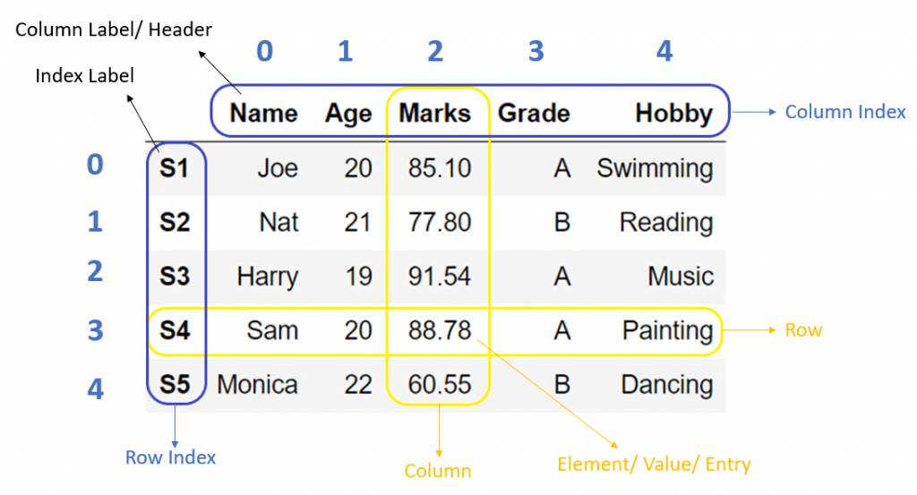
Dataframe is a tabular(rows, columns) representation of data. It is a two-dimensional data structure with potentially heterogeneous data.

Dataframe is a size-mutable structure that means data can be added or deleted from it, unlike data series, which does not allow operations that change its size.

DataFrame creation#

Data is available in various forms and types like CSV, SQL table, JSON, or Python structures like list, dict etc. We need to convert all such different data formats into a DataFrame so that we can use pandas libraries to analyze such data efficiently.

To create DataFrame, we can use either the DataFrame constructor or pandas built-in functions. Below are some examples.

DataFrame constructor#

pandas.DataFrame(data=None, index=None, columns=None, dtype=None, copy=False)

Parameters:#

data: It takes input dict, list, set, ndarray, iterable, or DataFrame. If the input is not provided, then it creates an empty DataFrame. The resultant column order follows the insertion order.
index: (Optional) It takes the list of row index for the DataFrame. The default value is a range of integers 0, 1,…n.
columns : (Optional) It takes the list of columns for the DataFrame. The default value is a range of integers 0, 1,…n.
dtype: (Optional) By default, It infers the data type from the data, but this option applies any specific data type to the whole DataFrame.
copy: (Optional) Copy data from inputs. Boolean, Default False. Only affects DataFrame or 2D array-like inputs

Refer the following articles for more details:

Dataframe from dict#

When we have data in dict or any default data structures in Python, we can convert it into DataFrame using the DataFrame constructor.

To construct a DataFrame from a dict object, we can pass it to the DataFrame constructor pd.DataFrame(dict). It creates DataFrame using, where dict keys will be column labels, and dict values will be the columns’ data. We can also use DataFrame.from_dict() function to Create DataFrame from dict.

Key and Imports:

Operator	Description
`df`	pandas DataFrame object
`s`	pandas Series object

# Example: 

student_dict = {'Name':['Joe','Nat'], 'Age':[20,21], 'Marks':[85.10, 77.80]}
student_dict

{'Name': ['Joe', 'Nat'], 'Age': [20, 21], 'Marks': [85.1, 77.8]}

‘Name’, ‘Age’ and ‘Marks’ are the keys in the dict when you convert they will become the column labels of the DataFrame.

import pandas as pd

# Python dict object
student_dict = {'Name': ['Joe', 'Nat'], 'Age': [20, 21], 'Marks': [85.10, 77.80]}
print(student_dict)

# Create DataFrame from dict
student_df = pd.DataFrame(student_dict)
print(student_df)

{'Name': ['Joe', 'Nat'], 'Age': [20, 21], 'Marks': [85.1, 77.8]}
  Name  Age  Marks
0  Joe   20   85.1
1  Nat   21   77.8

# Example

import pandas as pd

# We pass a dict of {column name: column values}
df = pd.DataFrame({'X':[78,85,96,80,86], 'Y':[84,94,89,83,86],'Z':[86,97,96,72,83]});
print(df)

# Example

import pandas as pd

df = pd.DataFrame({'A': [1, 2, 3], 'B': [True, True, False],
                   'C': [0.496714, -0.138264, 0.647689]},
                  index=['a', 'b', 'c'])  # also this weird index thing
df

	A	B	C
a	1	True	0.496714
b	2	True	-0.138264
c	3	False	0.647689

Indexing#

Our first improvement over numpy arrays is labeled indexing. We can select subsets by column, row, or both. Column selection uses the regular python __getitem__ machinery. Pass in a single column label 'A' or a list of labels ['A', 'C'] to select subsets of the original DataFrame.

# Single column, reduces to a Series
df['A']

a    1
b    2
c    3
Name: A, dtype: int64

cols = ['A', 'C']
df[cols]

	A	C
a	1	0.496714
b	2	-0.138264
c	3	0.647689

For row-wise selection, use the special .loc accessor.

df.loc[['a', 'b']]

	A	B	C
a	1	True	0.496714
b	2	True	-0.138264

You can use ranges to select rows or columns.

df.loc['a':'b']

	A	B	C
a	1	True	0.496714
b	2	True	-0.138264

Notice that the slice is inclusive on both sides, unlike your typical slicing of a list. Sometimes, you’d rather slice by position instead of label. .iloc has you covered:

df.iloc[[0, 1]]

	A	B	C
a	1	True	0.496714
b	2	True	-0.138264

df.iloc[:2]

	A	B	C
a	1	True	0.496714
b	2	True	-0.138264

This follows the usual python slicing rules: closed on the left, open on the right.

As I mentioned, you can slice both rows and columns. Use .loc for label or .iloc for position indexing.

df.loc['a', 'B']

True

Pandas, like NumPy, will reduce dimensions when possible. Select a single column and you get back Series (see below). Select a single row and single column, you get a scalar.

You can get pretty fancy:

df.loc['a':'b', ['A', 'C']]

	A	C
a	1	0.496714
b	2	-0.138264

Summary#

Use [] for selecting columns
Use .loc[row_lables, column_labels] for label-based indexing
Use .iloc[row_positions, column_positions] for positional index

I’ve left out boolean and hierarchical indexing, which we’ll see later.

Series#

You’ve already seen some Series up above. It’s the 1-dimensional analog of the DataFrame. Each column in a DataFrame is in some sense a Series. You can select a Series from a DataFrame in a few ways:

# __getitem__ like before
df['A']

a    1
b    2
c    3
Name: A, dtype: int64

# .loc, like before
df.loc[:, 'A']

a    1
b    2
c    3
Name: A, dtype: int64

# using `.` attribute lookup
df.A

a    1
b    2
c    3
Name: A, dtype: int64

df['mean'] = ['a', 'b', 'c']
df

	A	B	C	mean
a	1	True	0.496714	a
b	2	True	-0.138264	b
c	3	False	0.647689	c

df.mean

<bound method NDFrame._add_numeric_operations.<locals>.mean of    A      B         C mean
a  1   True  0.496714    a
b  2   True -0.138264    b
c  3  False  0.647689    c>

df['mean']

a    a
b    b
c    c
Name: mean, dtype: object

# Create DataSeries:

import pandas as pd
s = pd.Series([2, 4, 6, 8, 10])
print(s)

   2
   4
   6
   8
  10
dtype: int64

You’ll have to be careful with the last one. It won’t work if you’re column name isn’t a valid python identifier (say it has a space) or if it conflicts with one of the (many) methods on DataFrame. The . accessor is extremely convient for interactive use though.

You should never assign a column with . e.g. don’t do

# bad
df.A = [1, 2, 3]

It’s unclear whether your attaching the list [1, 2, 3] as an attribute of df, or whether you want it as a column. It’s better to just say

df['A'] = [1, 2, 3]
# or
df.loc[:, 'A'] = [1, 2, 3]

Series share many of the same methods as DataFrames.

Index#

Index are something of a peculiarity to pandas. First off, they are not the kind of indexes you’ll find in SQL, which are used to help the engine speed up certain queries. In pandas, Index are about lables. This helps with selection (like we did above) and automatic alignment when performing operations between two DataFrames or Series.

R does have row labels, but they’re nowhere near as powerful (or complicated) as in pandas. You can access the index of a DataFrame or Series with the .index attribute.

df.index

Index(['a', 'b', 'c'], dtype='object')

df.columns

Index(['A', 'B', 'C', 'mean'], dtype='object')

There are special kinds of Indexes that you’ll come across. Some of these are

MultiIndex for multidimensional (Hierarchical) labels
DatetimeIndex for datetimes
Float64Index for floats
CategoricalIndex for, you guessed it, Categoricals

How do you slice a DataFrame by row label?
- Use .loc[label]. For position based use .iloc[integer].
How do you select a column of a DataFrame?
- Standard __getitem__: df[column_name]
Is the Index a column in the DataFrame?
- No. It isn’t included in any operations (mean, etc). It can be inserted as a regular column with df.reset_index().

Dataframe from CSV#

In the field of Data Science, CSV files are used to store large datasets. To efficiently analyze such datasets, we need to convert them into pandas DataFrame.

To create a DataFrame from CSV, we use the read_csv('file_name') function that takes the file name as input and returns DataFrame as output.

Example 1:

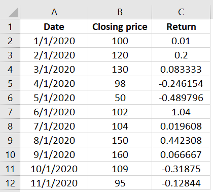
Let’s see how to read the stockprice_data.csv file into the DataFrame and then convert it into Pandas Series

import pandas as pd
data = pd.read_csv("stockprice_data.csv")
data

	Date	Closing price	Return
0	1/1/2020	100	0.010000
1	2/1/2020	120	0.200000
2	3/1/2020	130	0.083333
3	4/1/2020	98	-0.246154
4	5/1/2020	50	-0.489796
5	6/1/2020	102	1.040000
6	7/1/2020	104	0.019608
7	8/1/2020	150	0.442308
8	9/1/2020	160	0.066667
9	10/1/2020	109	-0.318750
10	11/1/2020	95	-0.128440

type(data)

pandas.core.frame.DataFrame

data1 = data.iloc[:,2]     # Convert Pandas Data Frame in to Pandas Series
data1

   0.010000
   0.200000
   0.083333
  -0.246154
  -0.489796
   1.040000
   0.019608
   0.442308
   0.066667
  -0.318750
 -0.128440
Name: Return, dtype: float64

type(data1)

pandas.core.series.Series

Example 2:

Let’s see how to read the automobile_data.csv file into the DataFrame.

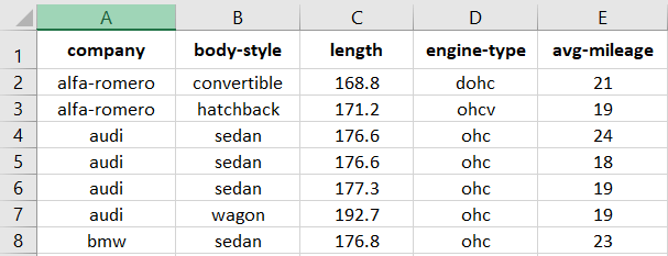
cars = pd.read_csv("automobile_data.csv")  # just give the name of file only if the file is in the same folder.
print(cars)

    index      company   body-style  wheel-base  length engine-type  \
     0  alfa-romero  convertible        88.6   168.8        dohc   
     1  alfa-romero  convertible        88.6   168.8        dohc   
     2  alfa-romero    hatchback        94.5   171.2        ohcv   
     3         audi        sedan        99.8   176.6         ohc   
     4         audi        sedan        99.4   176.6         ohc   
..    ...          ...          ...         ...     ...         ...   
   81   volkswagen        sedan        97.3   171.7         ohc   
   82   volkswagen        sedan        97.3   171.7         ohc   
   86   volkswagen        sedan        97.3   171.7         ohc   
   87        volvo        sedan       104.3   188.8         ohc   
   88        volvo        wagon       104.3   188.8         ohc   

   num-of-cylinders  horsepower  average-mileage    price  
            four         111               21  13495.0  
            four         111               21  16500.0  
             six         154               19  16500.0  
            four         102               24  13950.0  
            five         115               18  17450.0  
..              ...         ...              ...      ...  
           four          85               27   7975.0  
           four          52               37   7995.0  
           four         100               26   9995.0  
           four         114               23  12940.0  
           four         114               23  13415.0  

[61 rows x 10 columns]

DataFrame Options#

When DataFrame is vast, and we can not display the whole data while printing. In that case, we need to change how DataFrame gets display on the console using the print() function. For that, pandas have provided many options and functions to customize the presentation of the DataFrame.

To customize the display of DataFrame while printing#

When we display the DataFrame using print() function by default, it displays 10 rows (top 5 and bottom 5). Sometimes we may need to show more or lesser rows than the default view of the DataFrame.

We can change the setting by using pd.options or pd.set_option() functions. Both can be used interchangeably.

The below example will show a maximum of 20 and a minimum of 5 rows while printing DataFrame.

import pandas as pd

# Setting maximum rows to be shown 
pd.options.display.max_rows = 20

# Setting minimum rows to be shown
pd.set_option("display.min_rows", 5)

# Print DataFrame
print(cars)

    index      company   body-style  wheel-base  length engine-type  \
0       0  alfa-romero  convertible        88.6   168.8        dohc   
1       1  alfa-romero  convertible        88.6   168.8        dohc   
..    ...          ...          ...         ...     ...         ...   
59     87        volvo        sedan       104.3   188.8         ohc   
60     88        volvo        wagon       104.3   188.8         ohc   

   num-of-cylinders  horsepower  average-mileage    price  
0              four         111               21  13495.0  
1              four         111               21  16500.0  
..              ...         ...              ...      ...  
59             four         114               23  12940.0  
60             four         114               23  13415.0  

[61 rows x 10 columns]

DataFrame metadata#

Sometimes we need to get metadata of the DataFrame and not the content inside it. Such metadata information is useful to understand the DataFrame as it gives more details about the DataFrame that we need to process.

In this section, we cover the functions which provide such information of the DataFrame.

Let’s take an example of student DataFrame which contains ‘Name’, ‘Age’ and ‘Marks’ of students as shown below:

    Name  Age  Marks
  Joe   20  85.10
  Nat   21  77.80
Harry   19  91.54

Metadata info of DataFrame#

DataFrame.info() is a function of DataFrame that gives metadata of DataFrame. Which includes,

Number of rows and its range of index
Total number of columns
List of columns
Count of the total number of non-null values in the column
Data type of column
Count of columns in each data type
Memory usage by the DataFrame

# Example: In the below example, we got metadata information of student DataFrame.

# get dataframe info
student_df.info()

<class 'pandas.core.frame.DataFrame'>
RangeIndex: 2 entries, 0 to 1
Data columns (total 3 columns):
 #   Column  Non-Null Count  Dtype  
---  ------  --------------  -----  
 0   Name    2 non-null      object 
 1   Age     2 non-null      int64  
 2   Marks   2 non-null      float64
dtypes: float64(1), int64(1), object(1)
memory usage: 176.0+ bytes

Get the statistics of DataFrame#

DataFrame.describe() is a function that gives mathematical statistics of the data in DataFrame. But, it applies to the columns that contain numeric values.

In our example of student DataFrame, it gives descriptive statistics of ‘Age’ and ‘Marks’ columns only, that includes:

count: Total number of non-null values in the column
mean: an average of numbers
std: a standard deviation value
min: minimum value
25%: 25th percentile
50%: 50th percentile
75%: 75th percentile
max: maximum value

Note: Output of DataFrame.describe() function varies depending on the input DataFrame.

# Example

# get dataframe description
student_df.describe()

	Age	Marks
count	2.000000	2.00000
mean	20.500000	81.45000
std	0.707107	5.16188
min	20.000000	77.80000
25%	20.250000	79.62500
50%	20.500000	81.45000
75%	20.750000	83.27500
max	21.000000	85.10000

DataFrame Attributes#

DataFrame has provided many built-in attributes. Attributes do not modify the underlying data, unlike functions, but it is used to get more details about the DataFrame.

Following are majorly used attributes of the DataFrame:

Attribute	Description
`DataFrame.index`	It gives the Range of the row index
`DataFrame.columns`	It gives a list of column labels
`DataFrame.dtypes`	It gives column names and their data type
`DataFrame.values`	It gives all the rows in DataFrame
`DataFrame.empty`	It is used to check if the DataFrame is empty
`DataFrame.size`	It gives a total number of values in DataFrame
`DataFrame.shape`	It a number of rows and columns in DataFrame

# Example:

import pandas as pd

# Create DataFrame from dict
student_dict = {'Name': ['Joe', 'Nat', 'Harry'], 'Age': [20, 21, 19], 'Marks': [85.10, 77.80, 91.54]}

student_df = pd.DataFrame(student_dict)

print("DataFrame : ", student_df)

print("DataFrame Index : ", student_df.index)
print("DataFrame Columns : ", student_df.columns)

print("DataFrame Column types : ", student_df.dtypes)

print("DataFrame is empty? : ", student_df.empty)

print("DataFrame Shape : ", student_df.shape)
print("DataFrame Size : ", student_df.size)

print("DataFrame Values : ", student_df.values)

DataFrame :      Name  Age  Marks
0    Joe   20  85.10
1    Nat   21  77.80
2  Harry   19  91.54
DataFrame Index :  RangeIndex(start=0, stop=3, step=1)
DataFrame Columns :  Index(['Name', 'Age', 'Marks'], dtype='object')
DataFrame Column types :  Name      object
Age        int64
Marks    float64
dtype: object
DataFrame is empty? :  False
DataFrame Shape :  (3, 3)
DataFrame Size :  9
DataFrame Values :  [['Joe' 20 85.1]
 ['Nat' 21 77.8]
 ['Harry' 19 91.54]]

DataFrame selection#

While dealing with the vast data in DataFrame, a data analyst always needs to select a particular row or column for the analysis. In such cases, functions that can choose a set of rows or columns like top rows, bottom rows, or data within an index range play a significant role.

Following are the functions that help in selecting the subset of the DataFrame:

Attribute	Description
`DataFrame.head(n)`	It is used to select top ‘n’ rows in DataFrame.
`DataFrame.tail(n)`	It is used to select bottom ‘n’ rows in DataFrame.
`DataFrame.at`	It is used to get and set the particular value of DataFrame using row and column labels.
`DataFrame.iat`	It is used to get and set the particular value of DataFrame using row and column index positions.
`DataFrame.get(key)`	It is used to get the value of a key in DataFrame where Key is the column name.
`DataFrame.loc()`	It is used to select a group of data based on the row and column labels. It is used for slicing and filtering of the DataFrame.
`DataFrame.iloc()`	It is used to select a group of data based on the row and column index position. Use it for slicing and filtering the DataFrame.

# Example

import pandas as pd

# Create DataFrame from dict
student_dict = {'Name': ['Joe', 'Nat', 'Harry'], 'Age': [20, 21, 19], 'Marks': [85.10, 77.80, 91.54]}

student_df = pd.DataFrame(student_dict)

# display dataframe
print("DataFrame : ", student_df)

# select top 2 rows
print(student_df.head(2))

# select bottom 2 rows
print(student_df.tail(2))

# select value at row index 0 and column 'Name'
print(student_df.at[0, 'Name'])

# select value at first row and first column
print(student_df.iat[0, 0])

# select values of 'Name' column
print(student_df.get('Name'))

# select values from row index 0 to 2 and 'Name' column
print(student_df.loc[0:2, ['Name']])

# select values from row index 0 to 2(exclusive) and column position 0 to 2(exclusive)
print(student_df.iloc[0:2, 0:2])

DataFrame :      Name  Age  Marks
0    Joe   20  85.10
1    Nat   21  77.80
2  Harry   19  91.54
  Name  Age  Marks
0  Joe   20   85.1
1  Nat   21   77.8
    Name  Age  Marks
1    Nat   21  77.80
2  Harry   19  91.54
Joe
Joe
0      Joe
1      Nat
2    Harry
Name: Name, dtype: object
    Name
0    Joe
1    Nat
2  Harry
  Name  Age
0  Joe   20
1  Nat   21

DataFrame modification#

DataFrame is similar to any excel sheet or a database table where we need to insert new data or drop columns and rows if not required. Such data manipulation operations are very common on a DataFrame.

In this section, we discuss the data manipulation functions of the DataFrame.

Insert columns#

Sometimes it is required to add a new column in the DataFrame. DataFrame.insert() function is used to insert a new column in DataFrame at the specified position.

In the below example, we insert a new column ‘Class’ as a third new column in the DataFrame with default value ‘A’ using the syntax:

df.insert(loc = col_position, column = new_col_name, value = default_value)

# Example:

import pandas as pd

# Create DataFrame from dict
student_dict = {'Name': ['Joe', 'Nat', 'Harry'], 'Age': [20, 21, 19], 'Marks': [85.10, 77.80, 91.54]}
student_df = pd.DataFrame(student_dict)
print(student_df)

# insert new column in dataframe and display
student_df.insert(loc=2, column="Class", value='A')
print(student_df)

    Name  Age  Marks
  Joe   20  85.10
  Nat   21  77.80
Harry   19  91.54
    Name  Age Class  Marks
  Joe   20     A  85.10
  Nat   21     A  77.80
Harry   19     A  91.54

Drop columns#

DataFrame may contain redundant data, in such cases, we may need to delete such data that is not required. DataFrame.drop() function is used to delete the columns from DataFrame.

Refer to the following articles to get more details

Drop duplicates
Drop columns with NA

In the below example, we delete the “Age” column from the student DataFrame using df.drop(columns=[col1,col2...]).

import pandas as pd

# Create DataFrame from dict
student_dict = {'Name': ['Joe', 'Nat', 'Harry'], 'Age': [20, 21, 19], 'Marks': [85.10, 77.80, 91.54]}

student_df = pd.DataFrame(student_dict)
print(student_df)

# delete column from dataframe
student_df = student_df.drop(columns='Age')
print(student_df)

    Name  Age  Marks
  Joe   20  85.10
  Nat   21  77.80
Harry   19  91.54
    Name  Marks
  Joe  85.10
  Nat  77.80
Harry  91.54

Apply condition#

We may need to update the value in the DataFrame based on some condition. **DataFrame.where() **function is used to replace the value of DataFrame, where the condition is False.

Syntax:

where(filter, other=new_value)

It applies the filter condition on all the rows in the DataFrame, as follows:

If the filter condition returns False, then it updates the row with the value specified in other parameter.
If the filter condition returns True, then it does not update the row.

In the below example, we want to replace the student marks with ‘0’ where marks are less than 80. We pass a filter condition df['Marks'] > 80 to the function.

import pandas as pd

# Create DataFrame from dict
student_dict = {'Name': ['Joe', 'Nat', 'Harry'], 'Age': [20, 21, 19], 'Marks': [85.10, 77.80, 91.54]}

student_df = pd.DataFrame(student_dict)
print(student_df)

# Define filter condition
filter = student_df['Marks'] > 80

student_df['Marks'].where(filter, other=0, inplace=True)
print(student_df)

    Name  Age  Marks
  Joe   20  85.10
  Nat   21  77.80
Harry   19  91.54
    Name  Age  Marks
  Joe   20  85.10
  Nat   21   0.00
Harry   19  91.54

DataFrame filter columns#

Datasets contain massive data that need to be analyzed. But, sometimes, we may want to analyze relevant data and filter out all the other data. In such a case, we can use DataFrame.filter() function to fetch only required data from DataFrame.

It returns the subset of the DataFrame by applying conditions on each row index or column label as specified using the below syntax.

Syntax:

df.filter(like = filter_cond, axis = 'columns' or 'index')

It applies the condition on each row index or column label.

If the condition passed then, it includes that row or column in the resultant DataFrame.
If the condition failed, then it does not have that row or column in the resulting DataFrame.

Note: It applies the filter on row index or column label, not on actual data.

In the below example, we only include the column with a column label that starts with ‘N’.

import pandas as pd

# Create DataFrame from dict
student_dict = {'Name': ['Joe', 'Nat', 'Harry'], 'Age': [20, 21, 19], 'Marks': [85.10, 77.80, 91.54]}

student_df = pd.DataFrame(student_dict)
print(student_df)

# apply filter on dataframe
student_df = student_df.filter(like='N', axis='columns')
print(student_df)

    Name  Age  Marks
  Joe   20  85.10
  Nat   21  77.80
Harry   19  91.54
    Name
  Joe
  Nat
Harry

DataFrame rename columns#

While working with DataFrame, we may need to rename the column or row index. We can use DataFrame.rename() function to alter the row or column labels.

We need to pass a dictionary of key-value pairs as input to the function. Where key of the dict is the existing column label, and the value of dict is the new column label.

df.rename(columns = {'old':'new'})

It can be used to rename single or multiple columns and row labels.

In the below example, we rename column ‘Marks’ to ‘Percentage’ in the student DataFrame.

import pandas as pd

# Create DataFrame from dict
student_dict = {'Name': ['Joe', 'Nat', 'Harry'], 'Age': [20, 21, 19], 'Marks': [85.10, 77.80, 91.54]}

student_df = pd.DataFrame(student_dict)
print(student_df)

# rename column
student_df = student_df.rename(columns={'Marks': 'Percentage'})
print(student_df)

    Name  Age  Marks
  Joe   20  85.10
  Nat   21  77.80
Harry   19  91.54
    Name  Age  Percentage
  Joe   20       85.10
  Nat   21       77.80
Harry   19       91.54

DataFrame Join#

In most of the use cases of Data Analytics, data gathered from multiple sources, and we need to combine that data for further analysis. In such instances, join and merge operations are required.

DataFrame.join() function is used to join one DataFrame with another DataFrame as df1.join(df2)

In the below example, we joined two different DataFrames to create a new resultant DataFrame.

import pandas as pd

# create dataframe from dict 
student_dict = {'Name': ['Joe', 'Nat'], 'Age': [20, 21]}
student_df = pd.DataFrame(student_dict)
print(student_df)

# create dataframe from dict 
marks_dict = {'Marks': [85.10, 77.80]}
marks_df = pd.DataFrame(marks_dict)
print(marks_df)

# join dfs
joined_df = student_df.join(marks_df)
print(joined_df)

  Name  Age
0  Joe   20
1  Nat   21
   Marks
0   85.1
1   77.8
  Name  Age  Marks
0  Joe   20   85.1
1  Nat   21   77.8

DataFrame GroupBy#

GroupBy operation means splitting the data and then combining them based on some condition. Large data can be divided into logical groups to analyze it.

DataFrame.groupby() function groups the DataFrame row-wise or column-wise based on the condition.

If we want to analyze each class’s average marks, we need to combine the student data based on the ‘Class’ column and calculate its average using df.groupby(col_label).mean() as shown in the below example.

import pandas as pd

# Create DataFrame from dict
student_dict = {'Name': ['Joe', 'Nat', 'Harry'], 'Class': ['A', 'B', 'A'], 'Marks': [85.10, 77.80, 91.54]}
student_df = pd.DataFrame(student_dict)
print(student_df)

# apply group by 
student_df = student_df.groupby('Class').mean()
print(student_df)

    Name Class  Marks
0    Joe     A  85.10
1    Nat     B  77.80
2  Harry     A  91.54
       Marks
Class       
A      88.32
B      77.80

DataFrame Iteration#

DataFrame iteration means visiting each element in the DataFrame one by one. While analyzing a DataFrame, we may need to iterate over each row of the DataFrame.

There are multiple ways to iterate a DataFrame. We will see the function DataFrame.iterrows(), which can loop a DataFrame row-wise. It returns the index and row of the DataFrame in each iteration of the for a loop.

import pandas as pd

# Create DataFrame from dict
student_dict = {'Name': ['Joe', 'Nat'], 'Age': [20, 21], 'Marks': [85, 77]}
student_df = pd.DataFrame(student_dict)

# Iterate all the rows of DataFrame
for index, row in student_df.iterrows():
    print(index, row)

0 Name     Joe
Age       20
Marks     85
Name: 0, dtype: object
1 Name     Nat
Age       21
Marks     77
Name: 1, dtype: object

DataFrame Sorting#

Data Analyst always needs to perform different operations on the underlying data like merge, sort, concatenate, etc. The most frequently used operation is the sorting of data. Sorted data becomes easy to analyze and inferred.

The DataFrame.sort_values() function is used to sort the DataFrame using one or more columns in ascending (default) or descending order.

In the below example, we sort the student data based on the ‘Marks’.

import pandas as pd

# Create DataFrame from dict
student_dict = {'Name': ['Joe', 'Nat', 'Harry'], 'Age': [20, 21, 19], 'Marks': [85.10, 77.80, 91.54]}
student_df = pd.DataFrame(student_dict)
print(student_df)

# rename column
student_df = student_df.sort_values(by=['Marks'])
print(student_df)

    Name  Age  Marks
  Joe   20  85.10
  Nat   21  77.80
Harry   19  91.54
    Name  Age  Marks
  Nat   21  77.80
  Joe   20  85.10
Harry   19  91.54

DataFrame conversion#

After all the processing on DataFrame, we will get the expected data in the DataFrame. But, we may require to convert the DataFrame back to its original formats like CSV file or dict, or we may need to convert it to another format for further action like storing it into the Database as SQL table format.

Pandas have provided plenty of functions to convert the DataFrames into many different formats.

For example, DataFrame.to_dict() function is used to converts the DataFrame into a Python dictionary object.

Below is the example of a DataFrame which we need to convert into the Python dict.

    Name  Class Marks
  Joe     A  85.10
  Nat     B  77.80
Harry     A  91.54

Let’s see how we can use DataFrame.to_dict() function to convert the DataFrame into the Python dictionary. By default, it creates the dictionary with keys as column labels and values as mapping of the row index and data.

# convert dataframe to dict
dict = student_df.to_dict()
print(dict)

{'Name': {1: 'Nat', 0: 'Joe', 2: 'Harry'}, 'Age': {1: 21, 0: 20, 2: 19}, 'Marks': {1: 77.8, 0: 85.1, 2: 91.54}}

Summary:#

Create Test Objects#

Operator	Description
`pd.DataFrame(np.random.rand(20,5))`	5 columns and 20 rows of random floats
`pd.Series(my_list)`	Create a series from an iterable my_list
`df.index = pd.date_range('1900/1/30', periods=df.shape[0])`	Add a date index

Viewing/Inspecting Data#

Operator	Description
`df.head(n)`	First n rows of the DataFrame
`df.tail(n)`	Last n rows of the DataFrame
`df.shape`	Number of rows and columns
`df.info()`	Index, Datatype and Memory information
`df.describe()`	Summary statistics for numerical columns
`s.value_counts(dropna=False)`	View unique values and counts
`df.apply(pd.Series.value_counts)`	Unique values and counts for all columns

Selection#

Operator	Description
`df[col]`	Returns column with label col as Series
`df[[col1, col2]]`	Returns columns as a new DataFrame
`s.iloc[0]`	Selection by position
`s.loc['index_one']`	Selection by index
`df.iloc[0,:]`	First row
`df.iloc[0,0]`	First element of first column

Data Cleaning#

Operator	Description
`df.columns = ['a','b','c']`	Rename columns
`pd.isnull()`	Checks for null Values, Returns Boolean Arrray
`pd.notnull()`	Opposite of pd.isnull()
`df.dropna()`	Drop all rows that contain null values
`df.dropna(axis=1)`	Drop all columns that contain null values
`df.dropna(axis=1,thresh=n)`	Drop all rows have have less than n non null values
`df.fillna(x)`	Replace all null values with x
`s.fillna(s.mean())`	Replace all null values with the mean
`s.astype(float)`	Convert the datatype of the series to float
`s.replace(1,'one')`	Replace all values equal to 1 with ‘one’
`s.replace([2,3],['two', 'three'])`	Replace all 2 with ‘two’ and 3 with ‘three’
`df.rename(columns=lambda x: x + 1)`	Mass renaming of columns
`df.rename(columns={'old_name': 'new_ name'})`	Selective renaming
`df.set_index('column_one')`	Change the index
`df.rename(index=lambda x: x + 1)`	Mass renaming of index

Filter, Sort, and Groupby#

Operator	Description
`df[df[col] > 0.6]`	Rows where the column col is greater than 0.6
`df[(df[col] > 0.6) & (df[col] < 0.8)]`	Rows where 0.8 > col > 0.6
`df.sort_values(col1)`	Sort values by col1 in ascending order
`df.sort_values(col2,ascending=False)`	Sort values by col2 in descending order.5
`df.sort_values([col1,col2],ascending=[True,False])`	Sort values by col1 in ascending order then col2 in descending order
`df.groupby(col)`	Returns a groupby object for values from one column
`df.groupby([col1,col2])`	Returns groupby object for values from multiple columns
`df.groupby(col1)[col2]`	Returns the mean of the values in col2, grouped by the values in col1
`df.pivot_table(index=col1,values=[col2,col3],aggfunc=mean)`	Create a pivot table that groups by col1 and calculates the mean of col2 and col3
`df.groupby(col1).agg(np.mean)`	Find the average across all columns for every unique col1 group
`df.apply(np.mean)`	Apply the function np.mean() across each column
`nf.apply(np.max,axis=1)`	Apply the function np.max() across each row

Join/Combine#

Operator	Description
`df1.append(df2)`	Add the rows in df1 to the end of df2 (columns should be identical)
`pd.concat([df1, df2],axis=1)`	Add the columns in df1 to the end of df2 (rows should be identical)
`df1.join(df2,on=col1, how='inner')`	SQL-style join the columns in df1 with the columns on df2 where the rows for col have identical values. The ‘how’ can be ‘left’, ‘right’, ‘outer’ or ‘inner’

Statistics#

Operator	Description
`df.describe()`	Summary statistics for numerical columns
`df.mean()`	Returns the mean of all columns
`df.corr()`	Returns the correlation between columns in a DataFrame
`df.count()`	Returns the number of non-null values in each DataFrame column
`df.max()`	Returns the highest value in each column
`df.min()`	Returns the lowest value in each column
`df.median()`	Returns the median of each column
`df.std()`	Returns the standard deviation of each column

Importing Data#

Operator	Description
`pd.read_csv(filename)`	From a CSV file
`pd.read_table(filename)`	From a delimited text file (like TSV)
`pd.read_excel(filename)`	From an Excel file
`pd.read_sql(query, connection_object)`	Read from a SQL table/database
`pd.read_json(json_string)`	Read from a JSON formatted string, URL or file.
`pd.read_html(url)`	Parses an html URL, string or file and extracts tables to a list of dataframes
`pd.read_clipboard()`	Takes the contents of your clipboard and passes it to read_table()
`pd.DataFrame(dict)`	From a dict, keys for columns names, values for data as lists

Exporting Data#

Operator	Description
`df.to_csv(filename)`	Write to a CSV file
`df.to_excel(filename)`	Write to an Excel file
`df.to_sql(table_name, connection_object)`	Write to a SQL table
`df.to_json(filename)`	Write to a file in JSON format