PyTorch Transfer Learning

Note: This notebook uses torchvision’s new multi-weight support API (available in torchvision v0.13+).

We’ve built a few models by hand so far.

But their performance has been poor.

You might be thinking, is there a well-performing model that already exists for our problem?

And in the world of deep learning, the answer is often yes.

We’ll see how by using a powerful technique called transfer learning.

What is transfer learning?

Transfer learning allows us to take the patterns (also called weights) another model has learned from another problem and use them for our own problem.

For example, we can take the patterns a computer vision model has learned from datasets such as ImageNet (millions of images of different objects) and use them to power our FoodVision Mini model.

Or we could take the patterns from a language model (a model that’s been through large amounts of text to learn a representation of language) and use them as the basis of a model to classify different text samples.

The premise remains: find a well-performing existing model and apply it to your own problem.

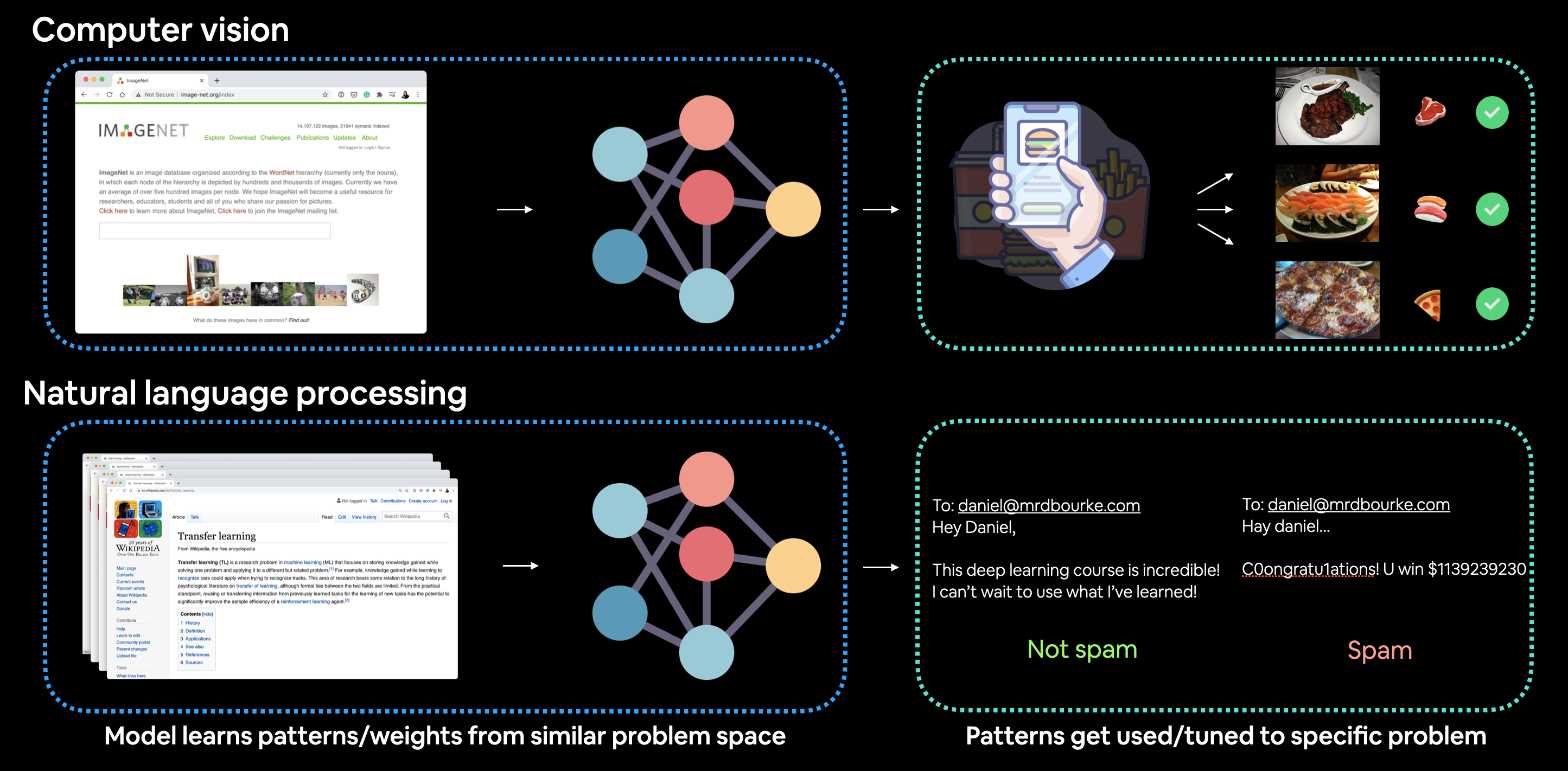
Example of transfer learning being applied to computer vision and natural language processing (NLP). In the case of computer vision, a computer vision model might learn patterns on millions of images in ImageNet and then use those patterns to infer on another problem. And for NLP, a language model may learn the structure of language by reading all of Wikipedia (and perhaps more) and then apply that knowledge to a different problem.

Why use transfer learning?

There are two main benefits to using transfer learning:

1. Can leverage an existing model (usually a neural network architecture) proven to work on problems similar to our own.

2. Can leverage a working model which has already learned patterns on similar data to our own. This often results in achieving great results with less custom data.

We’ll be putting these to the test for our FoodVision Mini problem, we’ll take a computer vision model pretrained on ImageNet and try to leverage its underlying learned representations for classifying images of pizza, steak and sushi.

Both research and practice support the use of transfer learning too.

A finding from a recent machine learning research paper recommended practioner’s use transfer learning wherever possible.

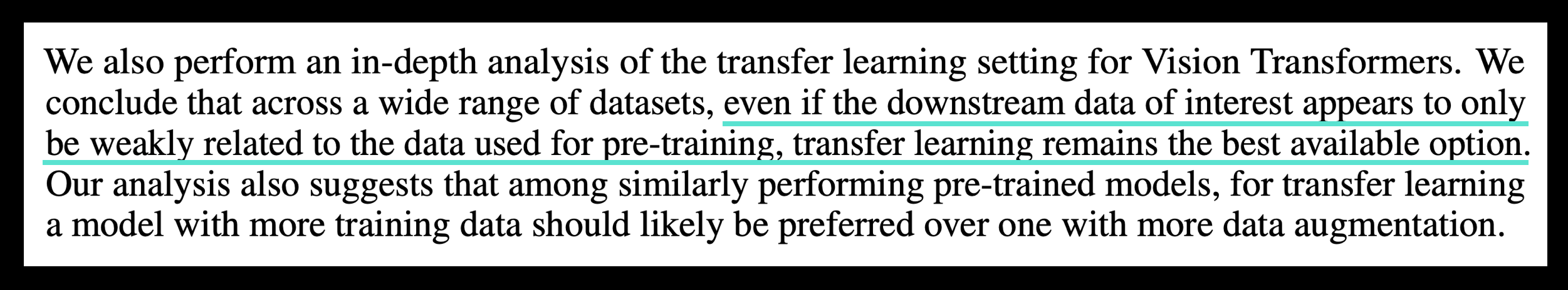
A study into the effects of whether training from scratch or using transfer learning was better from a practioner’s point of view, found transfer learning to be far more beneficial in terms of cost and time. Source: How to train your ViT? Data, Augmentation, and Regularization in Vision Transformers paper section 6 (conclusion).

And Jeremy Howard (founder of fastai) is a big proponent of transfer learning.

The things that really make a difference (transfer learning), if we can do better at transfer learning, it’s this world changing thing. Suddenly lots more people can do world-class work with less resources and less data. — Jeremy Howard on the Lex Fridman Podcast

Where to find pretrained models

The world of deep learning is an amazing place.

So amazing that many people around the world share their work.

Often, code and pretrained models for the latest state-of-the-art research is released within a few days of publishing.

And there are several places you can find pretrained models to use for your own problems.

Location	What’s there?	Link(s)
PyTorch domain libraries	Each of the PyTorch domain libraries (torchvision, torchtext) come with pretrained models of some form. The models there work right within PyTorch.	torchvision.models, torchtext.models, torchaudio.models, torchrec.models
HuggingFace Hub	A series of pretrained models on many different domains (vision, text, audio and more) from organizations around the world. There’s plenty of different datasets too.	https://huggingface.co/models, https://huggingface.co/datasets
timm (PyTorch Image Models) library	Almost all of the latest and greatest computer vision models in PyTorch code as well as plenty of other helpful computer vision features.	rwightman/pytorch-image-models
Paperswithcode	A collection of the latest state-of-the-art machine learning papers with code implementations attached. You can also find benchmarks here of model performance on different tasks.	https://paperswithcode.com/

With access to such high-quality resources as above, it should be common practice at the start of every deep learning problem you take on to ask, “Does a pretrained model exist for my problem?”

Exercise: Spend 5-minutes going through torchvision.models as well as the HuggingFace Hub Models page, what do you find? (there’s no right answers here, it’s just to practice exploring)

What we’re going to cover

We’re going to take a pretrained model from torchvision.models and customise it to work on (and hopefully improve) our FoodVision Mini problem.

Topic	Contents
Getting setup	We’ve written a fair bit of useful code over the past few sections, let’s download it and make sure we can use it again.
Get data	Let’s get the pizza, steak and sushi image classification dataset we’ve been using to try and improve our model’s results.
Create Datasets and DataLoaders	We’ll use the data_setup.py script we wrote in chapter 05. PyTorch Going Modular to setup our DataLoaders.
Get and customise a pretrained model	Here we’ll download a pretrained model from torchvision.models and customise it to our own problem.
Train model	Let’s see how the new pretrained model goes on our pizza, steak, sushi dataset. We’ll use the training functions we created in the previous chapter.
Evaluate the model by plotting loss curves	How did our first transfer learning model go? Did it overfit or underfit?
Make predictions on images from the test set	It’s one thing to check out a model’s evaluation metrics but it’s another thing to view its predictions on test samples, let’s visualize, visualize, visualize!

Where can you get help?

All of the materials for this course are available on GitHub.

If you run into trouble, you can ask a question on the course GitHub Discussions page.

And of course, there’s the PyTorch documentation and PyTorch developer forums, a very helpful place for all things PyTorch.

Getting setup

Let’s get started by importing/downloading the required modules for this section.

To save us writing extra code, we’re going to be leveraging some of the Python scripts (such as data_setup.py and engine.py) we created in the previous section, PyTorch Going Modular.

We’ll also get the torchinfo package if it’s not available.

torchinfo will help later on to give us a visual representation of our model.

# For this notebook to run with updated APIs, we need torch 1.12+ and torchvision 0.13+
try:
    import torch
    import torchvision
    assert int(torch.__version__.split(".")[1]) >= 12, "torch version should be 1.12+"
    assert int(torchvision.__version__.split(".")[1]) >= 13, "torchvision version should be 0.13+"
    print(f"torch version: {torch.__version__}")
    print(f"torchvision version: {torchvision.__version__}")
except:
    print(f"[INFO] torch/torchvision versions not as required, installing nightly versions.")
    !pip3 install -U torch torchvision torchaudio --extra-index-url https://download.pytorch.org/whl/cu113
    import torch
    import torchvision
    print(f"torch version: {torch.__version__}")
    print(f"torchvision version: {torchvision.__version__}")

torch version: 1.13.0.dev20220620+cu113
torchvision version: 0.14.0.dev20220620+cu113

# Continue with regular imports
import matplotlib.pyplot as plt
import torch
import torchvision

from torch import nn
from torchvision import transforms

# Try to get torchinfo, install it if it doesn't work
try:
    from torchinfo import summary
except:
    print("[INFO] Couldn't find torchinfo... installing it.")
    !pip install -q torchinfo
    from torchinfo import summary

# Try to import the going_modular directory, download it from GitHub if it doesn't work
try:
    from going_modular.going_modular import data_setup, engine
except:
    # Get the going_modular scripts
    print("[INFO] Couldn't find going_modular scripts... downloading them from GitHub.")
    !git clone https://github.com/mrdbourke/pytorch-deep-learning
    !mv pytorch-deep-learning/going_modular .
    !rm -rf pytorch-deep-learning
    from going_modular.going_modular import data_setup, engine

Now let’s setup device agnostic code.

Note: If you’re using Google Colab, and you don’t have a GPU turned on yet, it’s now time to turn one on via Runtime -> Change runtime type -> Hardware accelerator -> GPU.

# Setup device agnostic code
device = "cuda" if torch.cuda.is_available() else "cpu"
device

'cuda'

Get data

Before we can start to use transfer learning, we’ll need a dataset.

To see how transfer learning compares to our previous attempts at model building, we’ll download the same dataset we’ve been using for FoodVision Mini.

Let’s write some code to download the pizza_steak_sushi.zip dataset from the course GitHub and then unzip it.

We can also make sure if we’ve already got the data, it doesn’t redownload.

import os
import zipfile

from pathlib import Path

import requests

# Setup path to data folder
data_path = Path("data/")
image_path = data_path / "pizza_steak_sushi"

# If the image folder doesn't exist, download it and prepare it... 
if image_path.is_dir():
    print(f"{image_path} directory exists.")
else:
    print(f"Did not find {image_path} directory, creating one...")
    image_path.mkdir(parents=True, exist_ok=True)
    
    # Download pizza, steak, sushi data
    with open(data_path / "pizza_steak_sushi.zip", "wb") as f:
        request = requests.get("https://github.com/mrdbourke/pytorch-deep-learning/raw/main/data/pizza_steak_sushi.zip")
        print("Downloading pizza, steak, sushi data...")
        f.write(request.content)

    # Unzip pizza, steak, sushi data
    with zipfile.ZipFile(data_path / "pizza_steak_sushi.zip", "r") as zip_ref:
        print("Unzipping pizza, steak, sushi data...") 
        zip_ref.extractall(image_path)

    # Remove .zip file
    os.remove(data_path / "pizza_steak_sushi.zip")

data/pizza_steak_sushi directory exists.

Now we’ve got the same dataset we’ve been using previously, a series of images of pizza, steak and sushi in standard image classification format.

Let’s now create paths to our training and test directories.

# Setup Dirs
train_dir = image_path / "train"
test_dir = image_path / "test"

Create Datasets and DataLoaders

Since we’ve downloaded the going_modular directory, we can use the data_setup.py script we created in section PyTorch Going Modular to prepare and setup our DataLoaders.

But since we’ll be using a pretrained model from torchvision.models, there’s a specific transform we need to prepare our images first.

Creating a transform for torchvision.models (manual creation)

Note: As of torchvision v0.13+, there’s an update to how data transforms can be created using torchvision.models. I’ve called the previous method “manual creation” and the new method “auto creation”. This notebook showcases both.

When using a pretrained model, it’s important that your custom data going into the model is prepared in the same way as the original training data that went into the model.

Prior to torchvision v0.13+, to create a transform for a pretrained model in torchvision.models, the documentation stated:

All pre-trained models expect input images normalized in the same way, i.e. mini-batches of 3-channel RGB images of shape (3 x H x W), where H and W are expected to be at least 224.

The images have to be loaded in to a range of [0, 1] and then normalized using mean = [0.485, 0.456, 0.406] and std = [0.229, 0.224, 0.225].

You can use the following transform to normalize:

normalize = transforms.Normalize(mean=[0.485, 0.456, 0.406],
                                 std=[0.229, 0.224, 0.225])

The good news is, we can achieve the above transformations with a combination of:

Transform number	Transform required	Code to perform transform
1	Mini-batches of size [batch_size, 3, height, width] where height and width are at least 224x224^.	torchvision.transforms.Resize() to resize images into [3, 224, 224]^ and torch.utils.data.DataLoader() to create batches of images.
2	Values between 0 & 1.	torchvision.transforms.ToTensor()
3	A mean of [0.485, 0.456, 0.406] (values across each colour channel).	torchvision.transforms.Normalize(mean=...) to adjust the mean of our images.
4	A standard deviation of [0.229, 0.224, 0.225] (values across each colour channel).	torchvision.transforms.Normalize(std=...) to adjust the standard deviation of our images.

Note: ^some pretrained models from torchvision.models in different sizes to [3, 224, 224], for example, some might take them in [3, 240, 240]. For specific input image sizes, see the documentation.

Question: Where did the mean and standard deviation values come from? Why do we need to do this?

These were calculated from the data. Specifically, the ImageNet dataset by taking the means and standard deviations across a subset of images.

We also don’t need to do this. Neural networks are usually quite capable of figuring out appropriate data distributions (they’ll calculate where the mean and standard deviations need to be on their own) but setting them at the start can help our networks achieve better performance quicker.

Let’s compose a series of torchvision.transforms to perform the above steps.

# Create a transforms pipeline manually (required for torchvision < 0.13)
manual_transforms = transforms.Compose([
    transforms.Resize((224, 224)), # 1. Reshape all images to 224x224 (though some models may require different sizes)
    transforms.ToTensor(), # 2. Turn image values to between 0 & 1 
    transforms.Normalize(mean=[0.485, 0.456, 0.406], # 3. A mean of [0.485, 0.456, 0.406] (across each colour channel)
                         std=[0.229, 0.224, 0.225]) # 4. A standard deviation of [0.229, 0.224, 0.225] (across each colour channel),
])

Now we’ve got a manually created series of transforms ready to prepare our images, let’s create training and testing DataLoaders.

We can create these using the create_dataloaders function from the data_setup.py script we created in PyTorch Going Modular Part 2.

We’ll set batch_size=32 so our model see’s mini-batches of 32 samples at a time.

And we can transform our images using the transform pipeline we created above by setting transform=manual_transforms.

Note: I’ve included this manual creation of transforms in this notebook because you may come across resources that use this style. It’s also important to note that because these transforms are manually created, they’re also infinitely customizable. So if you wanted to included data augmentation techniques in your transforms pipeline, you could.

# Create training and testing DataLoaders as well as get a list of class names
train_dataloader, test_dataloader, class_names = data_setup.create_dataloaders(train_dir=train_dir,
                                                                               test_dir=test_dir,
                                                                               transform=manual_transforms, # resize, convert images to between 0 & 1 and normalize them
                                                                               batch_size=32) # set mini-batch size to 32

train_dataloader, test_dataloader, class_names

(<torch.utils.data.dataloader.DataLoader at 0x7fa9429a3a60>,
 <torch.utils.data.dataloader.DataLoader at 0x7fa9429a37c0>,
 ['pizza', 'steak', 'sushi'])

Creating a transform for torchvision.models (auto creation)

As previously stated, when using a pretrained model, it’s important that your custom data going into the model is prepared in the same way as the original training data that went into the model.

Above we saw how to manually create a transform for a pretrained model.

But as of torchvision v0.13+, an automatic transform creation feature has been added.

When you setup a model from torchvision.models and select the pretrained model weights you’d like to use, for example, say we’d like to use:

weights = torchvision.models.EfficientNet_B0_Weights.DEFAULT

Where,

• EfficientNet_B0_Weights is the model architecture weights we’d like to use (there are many differnt model architecture options in torchvision.models).

• DEFAULT means the best available weights (the best performance in ImageNet).

  • Note: Depending on the model architecture you choose, you may also see other options such as IMAGENET_V1 and IMAGENET_V2 where generally the higher version number the better. Though if you want the best available, DEFAULT is the easiest option. See the torchvision.models documentation for more.

Let’s try it out.

# Get a set of pretrained model weights
weights = torchvision.models.EfficientNet_B0_Weights.DEFAULT # .DEFAULT = best available weights from pretraining on ImageNet
weights

EfficientNet_B0_Weights.IMAGENET1K_V1

And now to access the transforms assosciated with our weights, we can use the transforms() method.

This is essentially saying “get the data transforms that were used to train the EfficientNet_B0_Weights on ImageNet”.

# Get the transforms used to create our pretrained weights
auto_transforms = weights.transforms()
auto_transforms

ImageClassification(
    crop_size=[224]
    resize_size=[256]
    mean=[0.485, 0.456, 0.406]
    std=[0.229, 0.224, 0.225]
    interpolation=InterpolationMode.BICUBIC
)

Notice how auto_transforms is very similar to manual_transforms, the only difference is that auto_transforms came with the model architecture we chose, where as we had to create manual_transforms by hand.

The benefit of automatically creating a transform through weights.transforms() is that you ensure you’re using the same data transformation as the pretrained model used when it was trained.

However, the tradeoff of using automatically created transforms is a lack of customization.

We can use auto_transforms to create DataLoaders with create_dataloaders() just as before.

# Create training and testing DataLoaders as well as get a list of class names
train_dataloader, test_dataloader, class_names = data_setup.create_dataloaders(train_dir=train_dir,
                                                                               test_dir=test_dir,
                                                                               transform=auto_transforms, # perform same data transforms on our own data as the pretrained model
                                                                               batch_size=32) # set mini-batch size to 32

train_dataloader, test_dataloader, class_names

(<torch.utils.data.dataloader.DataLoader at 0x7fa942951460>,
 <torch.utils.data.dataloader.DataLoader at 0x7fa942951550>,
 ['pizza', 'steak', 'sushi'])

Getting a pretrained model

Alright, here comes the fun part!

Over the past few notebooks we’ve been building PyTorch neural networks from scratch.

And while that’s a good skill to have, our models haven’t been performing as well as we’d like.

That’s where transfer learning comes in.

The whole idea of transfer learning is to take an already well-performing model on a problem-space similar to yours and then customising it to your use case.

Since we’re working on a computer vision problem (image classification with FoodVision Mini), we can find pretrained classification models in torchvision.models.

Exploring the documentation, you’ll find plenty of common computer vision architecture backbones such as:

Architecuture backbone	Code
ResNet’s	torchvision.models.resnet18(), torchvision.models.resnet50()…
VGG (similar to what we used for TinyVGG)	torchvision.models.vgg16()
EfficientNet’s	torchvision.models.efficientnet_b0(), torchvision.models.efficientnet_b1()…
VisionTransformer (ViT’s)	torchvision.models.vit_b_16(), torchvision.models.vit_b_32()…
ConvNeXt	torchvision.models.convnext_tiny(), torchvision.models.convnext_small()…
More available in torchvision.models	torchvision.models...

Which pretrained model should you use?

It depends on your problem/the device you’re working with.

Generally, the higher number in the model name (e.g. efficientnet_b0() -> efficientnet_b1() -> efficientnet_b7()) means better performance but a larger model.

You might think better performance is always better, right?

That’s true but some better performing models are too big for some devices.

For example, say you’d like to run your model on a mobile-device, you’ll have to take into account the limited compute resources on the device, thus you’d be looking for a smaller model.

But if you’ve got unlimited compute power, as The Bitter Lesson states, you’d likely take the biggest, most compute hungry model you can.

Understanding this performance vs. speed vs. size tradeoff will come with time and practice.

For me, I’ve found a nice balance in the efficientnet_bX models.

As of May 2022, Nutrify (the machine learning powered app I’m working on) is powered by an efficientnet_b0.

Comma.ai (a company that makes open source self-driving car software) uses an efficientnet_b2 to learn a representation of the road.

Note: Even though we’re using efficientnet_bX, it’s important not to get too attached to any one architecture, as they are always changing as new research gets released. Best to experiment, experiment, experiment and see what works for your problem.

Setting up a pretrained model

The pretrained model we’re going to be using is torchvision.models.efficientnet_b0().

The architecture is from the paper EfficientNet: Rethinking Model Scaling for Convolutional Neural Networks.

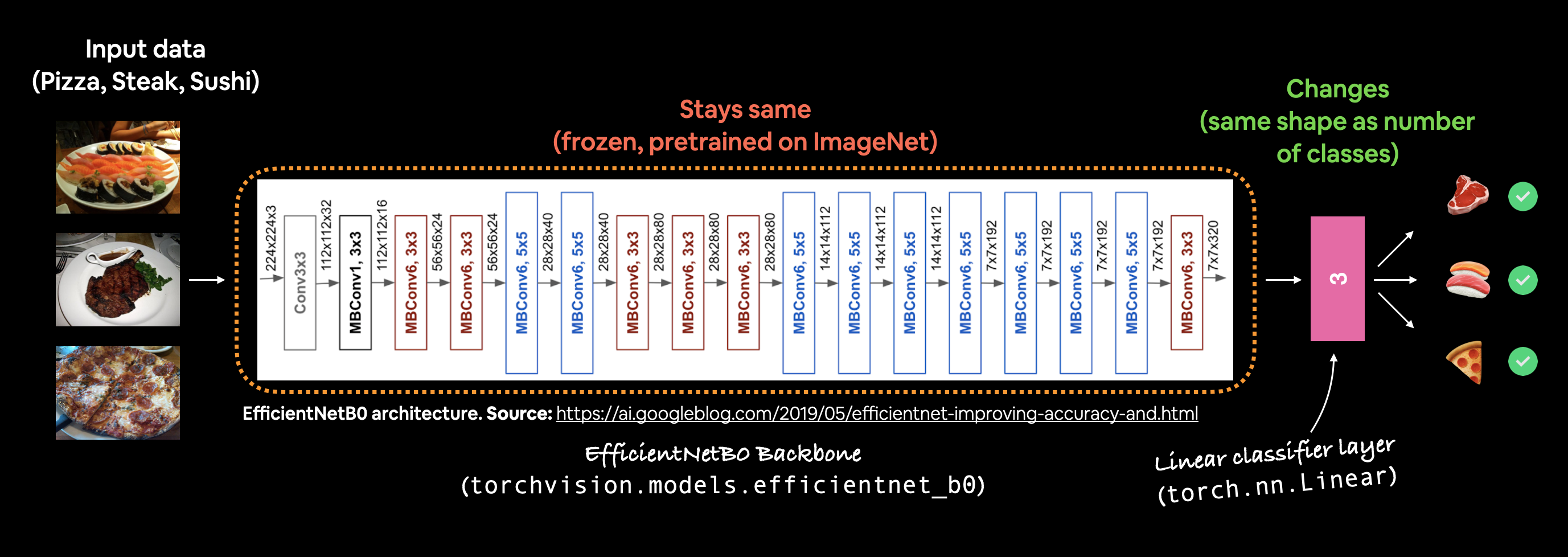
Example of what we’re going to create, a pretrained EfficientNet_B0 model from torchvision.models with the output layer adjusted for our use case of classifying pizza, steak and sushi images.

We can setup the EfficientNet_B0 pretrained ImageNet weights using the same code as we used to create the transforms.

weights = torchvision.models.EfficientNet_B0_Weights.DEFAULT # .DEFAULT = best available weights for ImageNet

This means the model has already been trained on millions of images and has a good base representation of image data.

The PyTorch version of this pretrained model is capable of achieving ~77.7% accuracy across ImageNet’s 1000 classes.

We’ll also send it to the target device.

# OLD: Setup the model with pretrained weights and send it to the target device (this was prior to torchvision v0.13)
# model = torchvision.models.efficientnet_b0(pretrained=True).to(device) # OLD method (with pretrained=True)

# NEW: Setup the model with pretrained weights and send it to the target device (torchvision v0.13+)
weights = torchvision.models.EfficientNet_B0_Weights.DEFAULT # .DEFAULT = best available weights 
model = torchvision.models.efficientnet_b0(weights=weights).to(device)

#model # uncomment to output (it's very long)

Note: In previous versions of torchvision, you’d create a pretrained model with code like:

model = torchvision.models.efficientnet_b0(pretrained=True).to(device)

However, running this using torchvision v0.13+ will result in errors such as the following:

UserWarning: The parameter 'pretrained' is deprecated since 0.13 and will be removed in 0.15, please use 'weights' instead.

And…

UserWarning: Arguments other than a weight enum or None for weights are deprecated since 0.13 and will be removed in 0.15. The current behavior is equivalent to passing weights=EfficientNet_B0_Weights.IMAGENET1K_V1. You can also use weights=EfficientNet_B0_Weights.DEFAULT to get the most up-to-date weights.

If we print the model, we get something similar to the following:

Lots and lots and lots of layers.

This is one of the benefits of transfer learning, taking an existing model, that’s been crafted by some of the best engineers in the world and applying to your own problem.

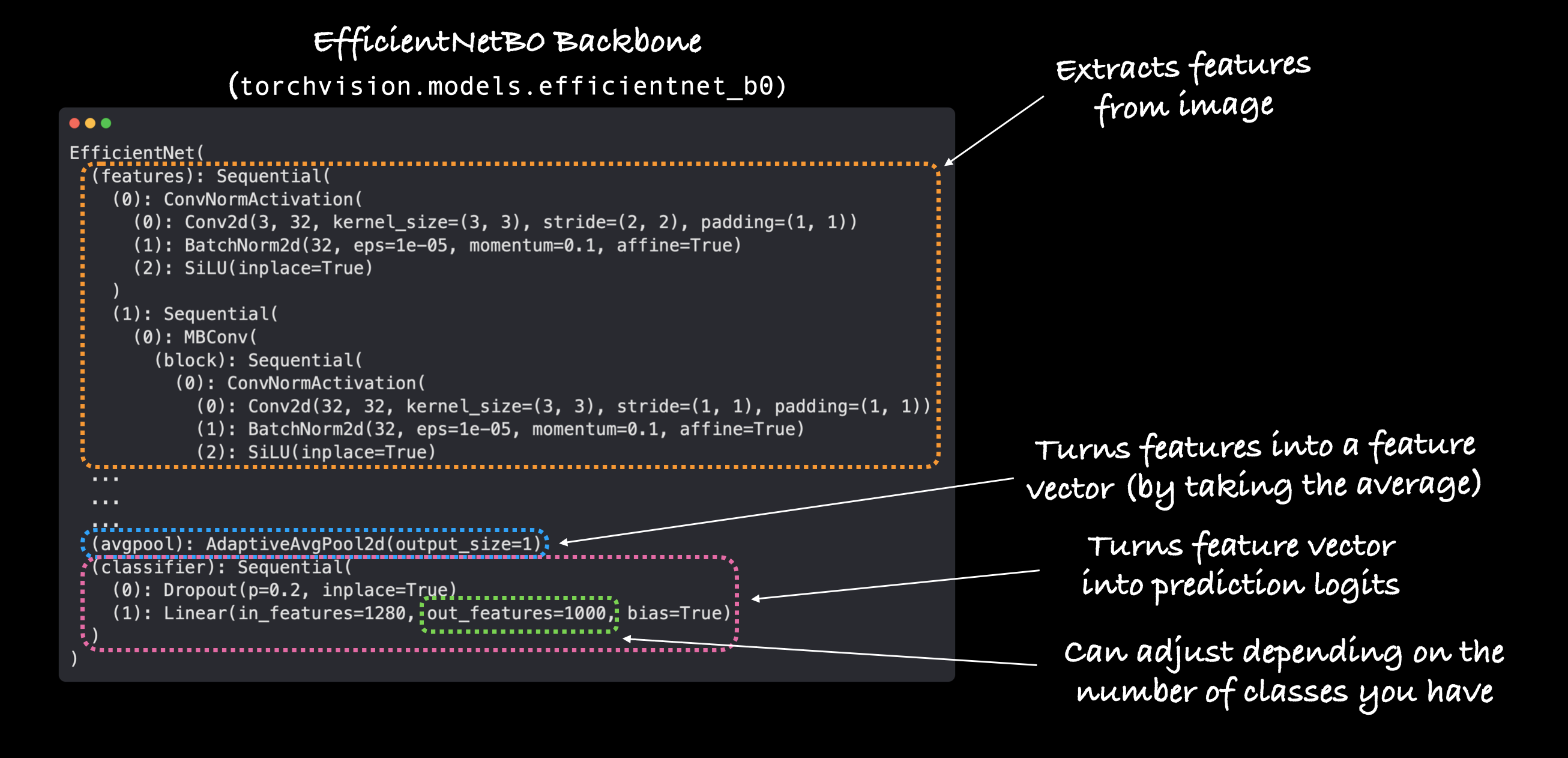
Our efficientnet_b0 comes in three main parts:

1. features - A collection of convolutional layers and other various activation layers to learn a base representation of vision data (this base representation/collection of layers is often referred to as features or feature extractor, “the base layers of the model learn the different features of images”).

2. avgpool - Takes the average of the output of the features layer(s) and turns it into a feature vector.

3. classifier - Turns the feature vector into a vector with the same dimensionality as the number of required output classes (since efficientnet_b0 is pretrained on ImageNet and because ImageNet has 1000 classes, out_features=1000 is the default).

Getting a summary of our model with torchinfo.summary()

To learn more about our model, let’s use torchinfo’s summary() method.

To do so, we’ll pass in:

• model - the model we’d like to get a summary of.

• input_size - the shape of the data we’d like to pass to our model, for the case of efficientnet_b0, the input size is (batch_size, 3, 224, 224), though other variants of efficientnet_bX have different input sizes.

  • Note: Many modern models can handle input images of varying sizes thanks to torch.nn.AdaptiveAvgPool2d(), this layer adaptively adjusts the output_size of a given input as required. You can try this out by passing different size input images to summary() or your models.

• col_names - the various information columns we’d like to see about our model.

• col_width - how wide the columns should be for the summary.

• row_settings - what features to show in a row.

# Print a summary using torchinfo (uncomment for actual output)
summary(model=model, 
        input_size=(32, 3, 224, 224), # make sure this is "input_size", not "input_shape"
        # col_names=["input_size"], # uncomment for smaller output
        col_names=["input_size", "output_size", "num_params", "trainable"],
        col_width=20,
        row_settings=["var_names"]
) 

============================================================================================================================================
Layer (type (var_name))                                      Input Shape          Output Shape         Param #              Trainable
============================================================================================================================================
EfficientNet (EfficientNet)                                  [32, 3, 224, 224]    [32, 1000]           --                   True
├─Sequential (features)                                      [32, 3, 224, 224]    [32, 1280, 7, 7]     --                   True
│    └─Conv2dNormActivation (0)                              [32, 3, 224, 224]    [32, 32, 112, 112]   --                   True
│    │    └─Conv2d (0)                                       [32, 3, 224, 224]    [32, 32, 112, 112]   864                  True
│    │    └─BatchNorm2d (1)                                  [32, 32, 112, 112]   [32, 32, 112, 112]   64                   True
│    │    └─SiLU (2)                                         [32, 32, 112, 112]   [32, 32, 112, 112]   --                   --
│    └─Sequential (1)                                        [32, 32, 112, 112]   [32, 16, 112, 112]   --                   True
│    │    └─MBConv (0)                                       [32, 32, 112, 112]   [32, 16, 112, 112]   1,448                True
│    └─Sequential (2)                                        [32, 16, 112, 112]   [32, 24, 56, 56]     --                   True
│    │    └─MBConv (0)                                       [32, 16, 112, 112]   [32, 24, 56, 56]     6,004                True
│    │    └─MBConv (1)                                       [32, 24, 56, 56]     [32, 24, 56, 56]     10,710               True
│    └─Sequential (3)                                        [32, 24, 56, 56]     [32, 40, 28, 28]     --                   True
│    │    └─MBConv (0)                                       [32, 24, 56, 56]     [32, 40, 28, 28]     15,350               True
│    │    └─MBConv (1)                                       [32, 40, 28, 28]     [32, 40, 28, 28]     31,290               True
│    └─Sequential (4)                                        [32, 40, 28, 28]     [32, 80, 14, 14]     --                   True
│    │    └─MBConv (0)                                       [32, 40, 28, 28]     [32, 80, 14, 14]     37,130               True
│    │    └─MBConv (1)                                       [32, 80, 14, 14]     [32, 80, 14, 14]     102,900              True
│    │    └─MBConv (2)                                       [32, 80, 14, 14]     [32, 80, 14, 14]     102,900              True
│    └─Sequential (5)                                        [32, 80, 14, 14]     [32, 112, 14, 14]    --                   True
│    │    └─MBConv (0)                                       [32, 80, 14, 14]     [32, 112, 14, 14]    126,004              True
│    │    └─MBConv (1)                                       [32, 112, 14, 14]    [32, 112, 14, 14]    208,572              True
│    │    └─MBConv (2)                                       [32, 112, 14, 14]    [32, 112, 14, 14]    208,572              True
│    └─Sequential (6)                                        [32, 112, 14, 14]    [32, 192, 7, 7]      --                   True
│    │    └─MBConv (0)                                       [32, 112, 14, 14]    [32, 192, 7, 7]      262,492              True
│    │    └─MBConv (1)                                       [32, 192, 7, 7]      [32, 192, 7, 7]      587,952              True
│    │    └─MBConv (2)                                       [32, 192, 7, 7]      [32, 192, 7, 7]      587,952              True
│    │    └─MBConv (3)                                       [32, 192, 7, 7]      [32, 192, 7, 7]      587,952              True
│    └─Sequential (7)                                        [32, 192, 7, 7]      [32, 320, 7, 7]      --                   True
│    │    └─MBConv (0)                                       [32, 192, 7, 7]      [32, 320, 7, 7]      717,232              True
│    └─Conv2dNormActivation (8)                              [32, 320, 7, 7]      [32, 1280, 7, 7]     --                   True
│    │    └─Conv2d (0)                                       [32, 320, 7, 7]      [32, 1280, 7, 7]     409,600              True
│    │    └─BatchNorm2d (1)                                  [32, 1280, 7, 7]     [32, 1280, 7, 7]     2,560                True
│    │    └─SiLU (2)                                         [32, 1280, 7, 7]     [32, 1280, 7, 7]     --                   --
├─AdaptiveAvgPool2d (avgpool)                                [32, 1280, 7, 7]     [32, 1280, 1, 1]     --                   --
├─Sequential (classifier)                                    [32, 1280]           [32, 1000]           --                   True
│    └─Dropout (0)                                           [32, 1280]           [32, 1280]           --                   --
│    └─Linear (1)                                            [32, 1280]           [32, 1000]           1,281,000            True
============================================================================================================================================
Total params: 5,288,548
Trainable params: 5,288,548
Non-trainable params: 0
Total mult-adds (G): 12.35
============================================================================================================================================
Input size (MB): 19.27
Forward/backward pass size (MB): 3452.35
Params size (MB): 21.15
Estimated Total Size (MB): 3492.77
============================================================================================================================================

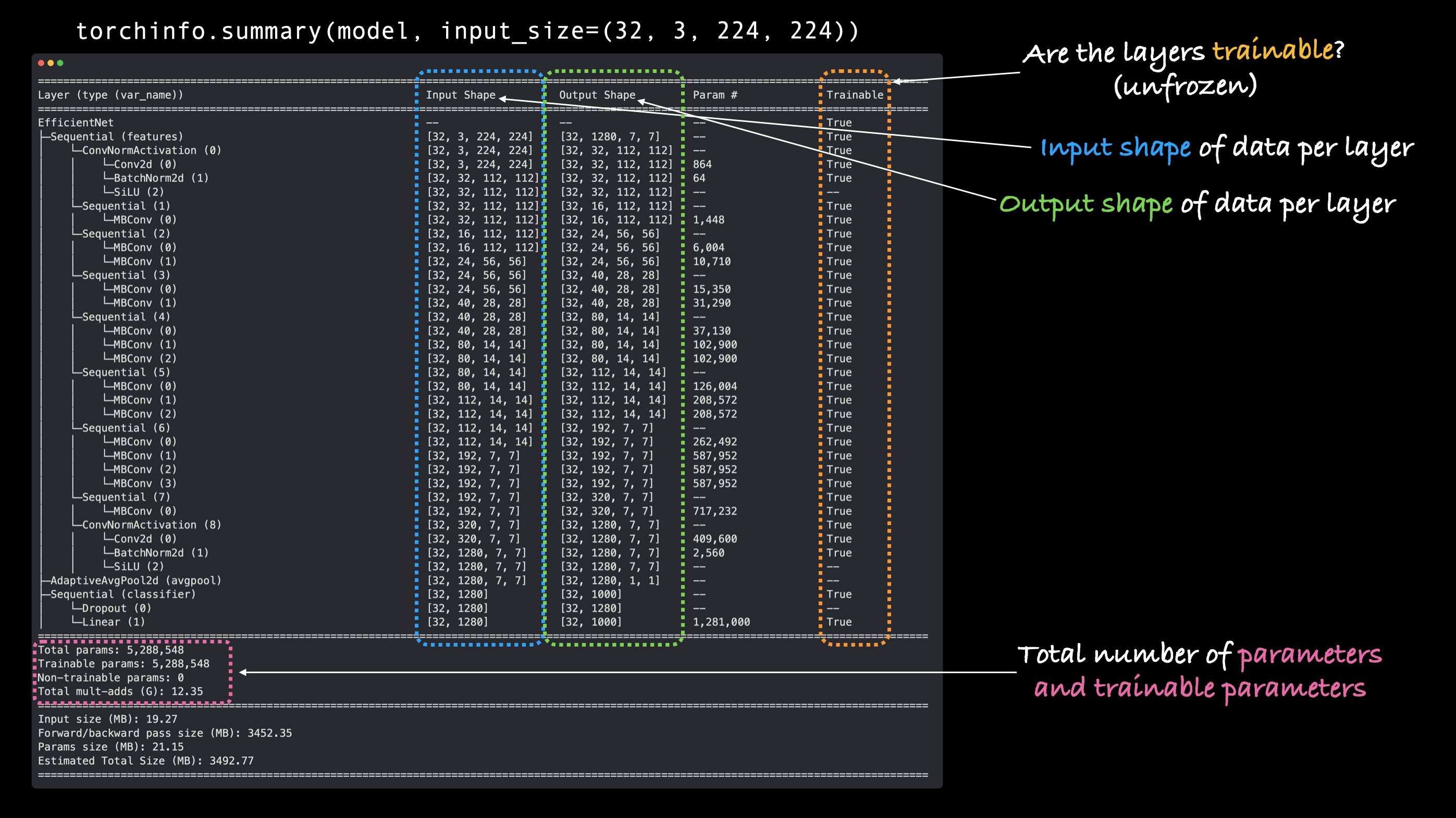
Woah!

Now that’s a big model!

From the output of the summary, we can see all of the various input and output shape changes as our image data goes through the model.

And there are a whole bunch more total parameters (pretrained weights) to recognize different patterns in our data.

For reference, our model from previous sections, TinyVGG had 8,083 parameters vs. 5,288,548 parameters for efficientnet_b0, an increase of ~654x!

What do you think, will this mean better performance?

Freezing the base model and changing the output layer to suit our needs

The process of transfer learning usually goes: freeze some base layers of a pretrained model (typically the features section) and then adjust the output layers (also called head/classifier layers) to suit your needs.

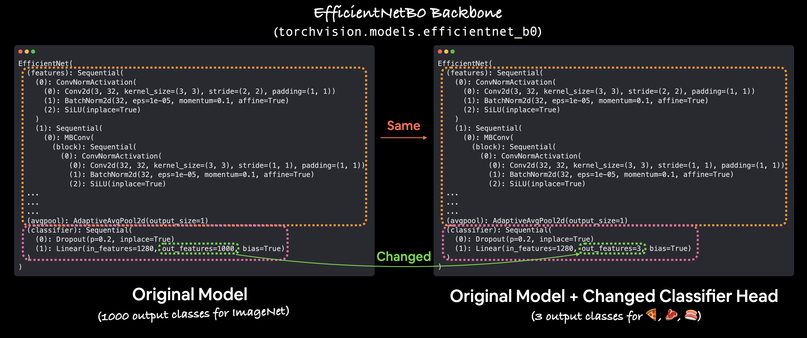
You can customise the outputs of a pretrained model by changing the output layer(s) to suit your problem. The original torchvision.models.efficientnet_b0() comes with out_features=1000 because there are 1000 classes in ImageNet, the dataset it was trained on. However, for our problem, classifying images of pizza, steak and sushi we only need out_features=3.

Let’s freeze all of the layers/parameters in the features section of our efficientnet_b0 model.

Note: To freeze layers means to keep them how they are during training. For example, if your model has pretrained layers, to freeze them would be to say, “don’t change any of the patterns in these layers during training, keep them how they are.” In essence, we’d like to keep the pretrained weights/patterns our model has learned from ImageNet as a backbone and then only change the output layers.

We can freeze all of the layers/parameters in the features section by setting the attribute requires_grad=False.

For parameters with requires_grad=False, PyTorch doesn’t track gradient updates and in turn, these parameters won’t be changed by our optimizer during training.

In essence, a parameter with requires_grad=False is “untrainable” or “frozen” in place.

# Freeze all base layers in the "features" section of the model (the feature extractor) by setting requires_grad=False
for param in model.features.parameters():
    param.requires_grad = False

Feature extractor layers frozen!

Let’s now adjust the output layer or the classifier portion of our pretrained model to our needs.

Right now our pretrained model has out_features=1000 because there are 1000 classes in ImageNet.

However, we don’t have 1000 classes, we only have three, pizza, steak and sushi.

We can change the classifier portion of our model by creating a new series of layers.

The current classifier consists of:

(classifier): Sequential(
    (0): Dropout(p=0.2, inplace=True)
    (1): Linear(in_features=1280, out_features=1000, bias=True)

We’ll keep the Dropout layer the same using torch.nn.Dropout(p=0.2, inplace=True).

Note: Dropout layers randomly remove connections between two neural network layers with a probability of p. For example, if p=0.2, 20% of connections between neural network layers will be removed at random each pass. This practice is meant to help regularize (prevent overfitting) a model by making sure the connections that remain learn features to compensate for the removal of the other connections (hopefully these remaining features are more general).

And we’ll keep in_features=1280 for our Linear output layer but we’ll change the out_features value to the length of our class_names (len(['pizza', 'steak', 'sushi']) = 3).

Our new classifier layer should be on the same device as our model.

# Set the manual seeds
torch.manual_seed(42)
torch.cuda.manual_seed(42)

# Get the length of class_names (one output unit for each class)
output_shape = len(class_names)

# Recreate the classifier layer and seed it to the target device
model.classifier = torch.nn.Sequential(
    torch.nn.Dropout(p=0.2, inplace=True), 
    torch.nn.Linear(in_features=1280, 
                    out_features=output_shape, # same number of output units as our number of classes
                    bias=True)).to(device)

Output layer updated, let’s get another summary of our model and see what’s changed.

# # Do a summary *after* freezing the features and changing the output classifier layer (uncomment for actual output)
summary(model, 
        input_size=(32, 3, 224, 224), # make sure this is "input_size", not "input_shape" (batch_size, color_channels, height, width)
        verbose=0,
        col_names=["input_size", "output_size", "num_params", "trainable"],
        col_width=20,
        row_settings=["var_names"]
)

============================================================================================================================================
Layer (type (var_name))                                      Input Shape          Output Shape         Param #              Trainable
============================================================================================================================================
EfficientNet (EfficientNet)                                  [32, 3, 224, 224]    [32, 3]              --                   Partial
├─Sequential (features)                                      [32, 3, 224, 224]    [32, 1280, 7, 7]     --                   False
│    └─Conv2dNormActivation (0)                              [32, 3, 224, 224]    [32, 32, 112, 112]   --                   False
│    │    └─Conv2d (0)                                       [32, 3, 224, 224]    [32, 32, 112, 112]   (864)                False
│    │    └─BatchNorm2d (1)                                  [32, 32, 112, 112]   [32, 32, 112, 112]   (64)                 False
│    │    └─SiLU (2)                                         [32, 32, 112, 112]   [32, 32, 112, 112]   --                   --
│    └─Sequential (1)                                        [32, 32, 112, 112]   [32, 16, 112, 112]   --                   False
│    │    └─MBConv (0)                                       [32, 32, 112, 112]   [32, 16, 112, 112]   (1,448)              False
│    └─Sequential (2)                                        [32, 16, 112, 112]   [32, 24, 56, 56]     --                   False
│    │    └─MBConv (0)                                       [32, 16, 112, 112]   [32, 24, 56, 56]     (6,004)              False
│    │    └─MBConv (1)                                       [32, 24, 56, 56]     [32, 24, 56, 56]     (10,710)             False
│    └─Sequential (3)                                        [32, 24, 56, 56]     [32, 40, 28, 28]     --                   False
│    │    └─MBConv (0)                                       [32, 24, 56, 56]     [32, 40, 28, 28]     (15,350)             False
│    │    └─MBConv (1)                                       [32, 40, 28, 28]     [32, 40, 28, 28]     (31,290)             False
│    └─Sequential (4)                                        [32, 40, 28, 28]     [32, 80, 14, 14]     --                   False
│    │    └─MBConv (0)                                       [32, 40, 28, 28]     [32, 80, 14, 14]     (37,130)             False
│    │    └─MBConv (1)                                       [32, 80, 14, 14]     [32, 80, 14, 14]     (102,900)            False
│    │    └─MBConv (2)                                       [32, 80, 14, 14]     [32, 80, 14, 14]     (102,900)            False
│    └─Sequential (5)                                        [32, 80, 14, 14]     [32, 112, 14, 14]    --                   False
│    │    └─MBConv (0)                                       [32, 80, 14, 14]     [32, 112, 14, 14]    (126,004)            False
│    │    └─MBConv (1)                                       [32, 112, 14, 14]    [32, 112, 14, 14]    (208,572)            False
│    │    └─MBConv (2)                                       [32, 112, 14, 14]    [32, 112, 14, 14]    (208,572)            False
│    └─Sequential (6)                                        [32, 112, 14, 14]    [32, 192, 7, 7]      --                   False
│    │    └─MBConv (0)                                       [32, 112, 14, 14]    [32, 192, 7, 7]      (262,492)            False
│    │    └─MBConv (1)                                       [32, 192, 7, 7]      [32, 192, 7, 7]      (587,952)            False
│    │    └─MBConv (2)                                       [32, 192, 7, 7]      [32, 192, 7, 7]      (587,952)            False
│    │    └─MBConv (3)                                       [32, 192, 7, 7]      [32, 192, 7, 7]      (587,952)            False
│    └─Sequential (7)                                        [32, 192, 7, 7]      [32, 320, 7, 7]      --                   False
│    │    └─MBConv (0)                                       [32, 192, 7, 7]      [32, 320, 7, 7]      (717,232)            False
│    └─Conv2dNormActivation (8)                              [32, 320, 7, 7]      [32, 1280, 7, 7]     --                   False
│    │    └─Conv2d (0)                                       [32, 320, 7, 7]      [32, 1280, 7, 7]     (409,600)            False
│    │    └─BatchNorm2d (1)                                  [32, 1280, 7, 7]     [32, 1280, 7, 7]     (2,560)              False
│    │    └─SiLU (2)                                         [32, 1280, 7, 7]     [32, 1280, 7, 7]     --                   --
├─AdaptiveAvgPool2d (avgpool)                                [32, 1280, 7, 7]     [32, 1280, 1, 1]     --                   --
├─Sequential (classifier)                                    [32, 1280]           [32, 3]              --                   True
│    └─Dropout (0)                                           [32, 1280]           [32, 1280]           --                   --
│    └─Linear (1)                                            [32, 1280]           [32, 3]              3,843                True
============================================================================================================================================
Total params: 4,011,391
Trainable params: 3,843
Non-trainable params: 4,007,548
Total mult-adds (G): 12.31
============================================================================================================================================
Input size (MB): 19.27
Forward/backward pass size (MB): 3452.09
Params size (MB): 16.05
Estimated Total Size (MB): 3487.41
============================================================================================================================================

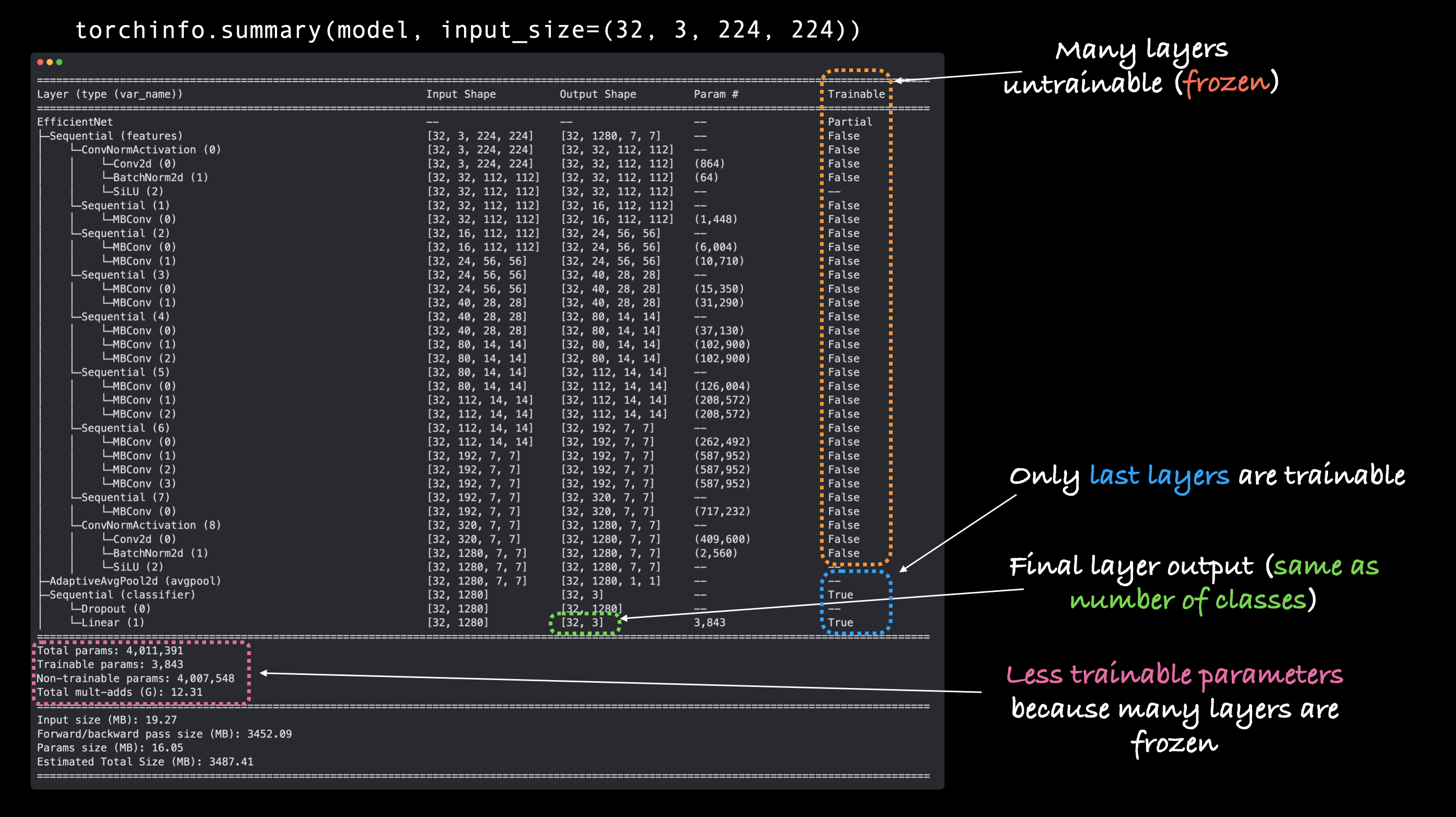
Ho, ho! There’s a fair few changes here!

Let’s go through them:

• Trainable column - You’ll see that many of the base layers (the ones in the features portion) have their Trainable value as False. This is because we set their attribute requires_grad=False. Unless we change this, these layers won’t be updated during furture training.

• Output shape of classifier - The classifier portion of the model now has an Output Shape value of [32, 3] instead of [32, 1000]. It’s Trainable value is also True. This means its parameters will be updated during training. In essence, we’re using the features portion to feed our classifier portion a base representation of an image and then our classifier layer is going to learn how to base representation aligns with our problem.

• Less trainable parameters - Previously there was 5,288,548 trainable parameters. But since we froze many of the layers of the model and only left the classifier as trainable, there’s now only 3,843 trainable parameters (even less than our TinyVGG model). Though there’s also 4,007,548 non-trainable parameters, these will create a base representation of our input images to feed into our classifier layer.

Note: The more trainable parameters a model has, the more compute power/longer it takes to train. Freezing the base layers of our model and leaving it with less trainable parameters means our model should train quite quickly. This is one huge benefit of transfer learning, taking the already learned parameters of a model trained on a problem similar to yours and only tweaking the outputs slightly to suit your problem.

Train model

Now we’ve got a pretrained model that’s semi-frozen and has a customised classifier, how about we see transfer learning in action?

To begin training, let’s create a loss function and an optimizer.

Because we’re still working with multi-class classification, we’ll use nn.CrossEntropyLoss() for the loss function.

And we’ll stick with torch.optim.Adam() as our optimizer with lr=0.001.

# Define loss and optimizer
loss_fn = nn.CrossEntropyLoss()
optimizer = torch.optim.Adam(model.parameters(), lr=0.001)

To train our model, we can use train() function we defined in the PyTorch Going Modular section 04.

The train() function is in the engine.py script inside the going_modular directory.

Let’s see how long it takes to train our model for 5 epochs.

Note: We’re only going to be training the parameters classifier here as all of the other parameters in our model have been frozen.

# Set the random seeds
torch.manual_seed(42)
torch.cuda.manual_seed(42)

# Start the timer
from timeit import default_timer as timer 
start_time = timer()

# Setup training and save the results
results = engine.train(model=model,
                       train_dataloader=train_dataloader,
                       test_dataloader=test_dataloader,
                       optimizer=optimizer,
                       loss_fn=loss_fn,
                       epochs=5,
                       device=device)

# End the timer and print out how long it took
end_time = timer()
print(f"[INFO] Total training time: {end_time-start_time:.3f} seconds")

Epoch: 1 | train_loss: 1.0924 | train_acc: 0.3984 | test_loss: 0.9133 | test_acc: 0.5398
Epoch: 2 | train_loss: 0.8717 | train_acc: 0.7773 | test_loss: 0.7912 | test_acc: 0.8153
Epoch: 3 | train_loss: 0.7648 | train_acc: 0.7930 | test_loss: 0.7463 | test_acc: 0.8561
Epoch: 4 | train_loss: 0.7108 | train_acc: 0.7539 | test_loss: 0.6372 | test_acc: 0.8655
Epoch: 5 | train_loss: 0.6254 | train_acc: 0.7852 | test_loss: 0.6260 | test_acc: 0.8561
[INFO] Total training time: 8.977 seconds

Our model trained quite fast (~5 seconds on my local machine with a NVIDIA TITAN RTX GPU/about 15 seconds on Google Colab with a NVIDIA P100 GPU).

And it looks like it smashed our previous model results out of the park!

With an efficientnet_b0 backbone, our model achieves almost 85%+ accuracy on the test dataset, almost double what we were able to achieve with TinyVGG.

Not bad for a model we downloaded with a few lines of code.

Evaluate model by plotting loss curves

Our model looks like it’s performing pretty well.

Let’s plot it’s loss curves to see what the training looks like over time.

We can plot the loss curves using the function plot_loss_curves() we created in PyTorch Custom Datasets section 7.8.

The function is stored in the helper_functions.py script so we’ll try to import it and download the script if we don’t have it.

# Get the plot_loss_curves() function from helper_functions.py, download the file if we don't have it
try:
    from helper_functions import plot_loss_curves
except:
    print("[INFO] Couldn't find helper_functions.py, downloading...")
    with open("helper_functions.py", "wb") as f:
        import requests
        request = requests.get("helper_functions.py")
        f.write(request.content)
    from helper_functions import plot_loss_curves

# Plot the loss curves of our model
plot_loss_curves(results)

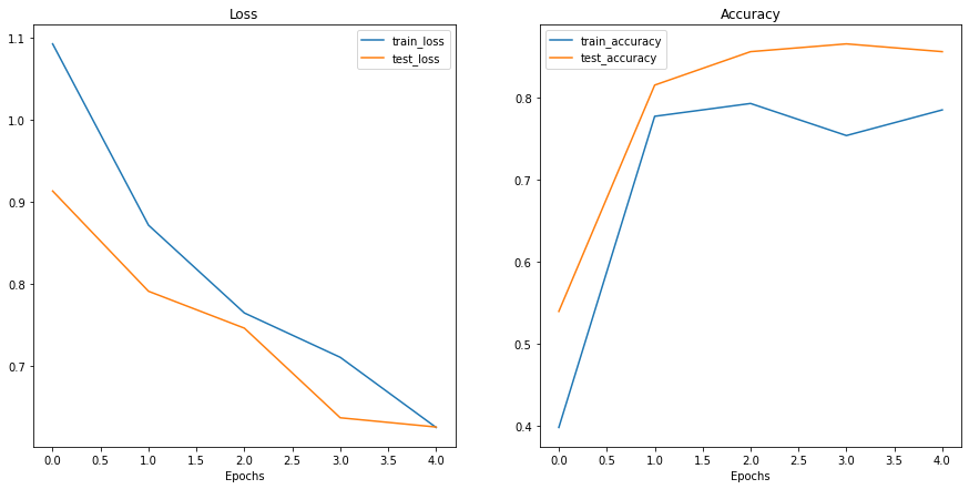
Those are some excellent looking loss curves!

It looks like the loss for both datasets (train and test) is heading in the right direction.

The same with the accuracy values, trending upwards.

That goes to show the power of transfer learning. Using a pretrained model often leads to pretty good results with a small amount of data in less time.

I wonder what would happen if you tried to train the model for longer? Or if we added more data?

Question: Looking at the loss curves, does our model look like it’s overfitting or underfitting? Or perhaps neither? Hint: Check out notebook PyTorch Custom Datasets part - What should an ideal loss curve look like? for ideas.

Make predictions on images from the test set

It looks like our model performs well quantitatively but how about qualitatively?

Let’s find out by making some predictions with our model on images from the test set (these aren’t seen during training) and plotting them.

Visualize, visualize, visualize!

One thing we’ll have to remember is that for our model to make predictions on an image, the image has to be in same format as the images our model was trained on.

This means we’ll need to make sure our images have:

• Same shape - If our images are different shapes to what our model was trained on, we’ll get shape errors.

• Same datatype - If our images are a different datatype (e.g. torch.int8 vs. torch.float32) we’ll get datatype errors.

• Same device - If our images are on a different device to our model, we’ll get device errors.

• Same transformations - If our model is trained on images that have been transformed in certain way (e.g. normalized with a specific mean and standard deviation) and we try and make preidctions on images transformed in a different way, these predictions may be off.

Note: These requirements go for all kinds of data if you’re trying to make predictions with a trained model. Data you’d like to predict on should be in the same format as your model was trained on.

To do all of this, we’ll create a function pred_and_plot_image() to:

1. Take in a trained model, a list of class names, a filepath to a target image, an image size, a transform and a target device.

2. Open an image with PIL.Image.open().

3. Create a transform for the image (this will default to the manual_transforms we created above or it could use a transform generated from weights.transforms()).

4. Make sure the model is on the target device.

5. Turn on model eval mode with model.eval() (this turns off layers like nn.Dropout(), so they aren’t used for inference) and the inference mode context manager.

6. Transform the target image with the transform made in step 3 and add an extra batch dimension with torch.unsqueeze(dim=0) so our input image has shape [batch_size, color_channels, height, width].

7. Make a prediction on the image by passing it to the model ensuring it’s on the target device.

8. Convert the model’s output logits to prediction probabilities with torch.softmax().

9. Convert model’s prediction probabilities to prediction labels with torch.argmax().

10. Plot the image with matplotlib and set the title to the prediction label from step 9 and prediction probability from step 8.

Note: This is a similar function to PyTorch Custom Datasets section 11.3’s pred_and_plot_image() with a few tweaked steps.

from typing import List, Tuple

from PIL import Image

# 1. Take in a trained model, class names, image path, image size, a transform and target device
def pred_and_plot_image(model: torch.nn.Module,
                        image_path: str, 
                        class_names: List[str],
                        image_size: Tuple[int, int] = (224, 224),
                        transform: torchvision.transforms = None,
                        device: torch.device=device):
    
    
    # 2. Open image
    img = Image.open(image_path)

    # 3. Create transformation for image (if one doesn't exist)
    if transform is not None:
        image_transform = transform
    else:
        image_transform = transforms.Compose([
            transforms.Resize(image_size),
            transforms.ToTensor(),
            transforms.Normalize(mean=[0.485, 0.456, 0.406],
                                 std=[0.229, 0.224, 0.225]),
        ])

    ### Predict on image ### 

    # 4. Make sure the model is on the target device
    model.to(device)

    # 5. Turn on model evaluation mode and inference mode
    model.eval()
    with torch.inference_mode():
      # 6. Transform and add an extra dimension to image (model requires samples in [batch_size, color_channels, height, width])
      transformed_image = image_transform(img).unsqueeze(dim=0)

      # 7. Make a prediction on image with an extra dimension and send it to the target device
      target_image_pred = model(transformed_image.to(device))

    # 8. Convert logits -> prediction probabilities (using torch.softmax() for multi-class classification)
    target_image_pred_probs = torch.softmax(target_image_pred, dim=1)

    # 9. Convert prediction probabilities -> prediction labels
    target_image_pred_label = torch.argmax(target_image_pred_probs, dim=1)

    # 10. Plot image with predicted label and probability 
    plt.figure()
    plt.imshow(img)
    plt.title(f"Pred: {class_names[target_image_pred_label]} | Prob: {target_image_pred_probs.max():.3f}")
    plt.axis(False);

What a good looking function!

Let’s test it out by making predictions on a few random images from the test set.

We can get a list of all the test image paths using list(Path(test_dir).glob("*/*.jpg")), the stars in the glob() method say “any file matching this pattern”, in other words, any file ending in .jpg (all of our images).

And then we can randomly sample a number of these using Python’s random.sample(populuation, k) where population is the sequence to sample and k is the number of samples to retrieve.

# Get a random list of image paths from test set
import random
num_images_to_plot = 3
test_image_path_list = list(Path(test_dir).glob("*/*.jpg")) # get list all image paths from test data 
test_image_path_sample = random.sample(population=test_image_path_list, # go through all of the test image paths
                                       k=num_images_to_plot) # randomly select 'k' image paths to pred and plot

# Make predictions on and plot the images
for image_path in test_image_path_sample:
    pred_and_plot_image(model=model, 
                        image_path=image_path,
                        class_names=class_names,
                        # transform=weights.transforms(), # optionally pass in a specified transform from our pretrained model weights
                        image_size=(224, 224))

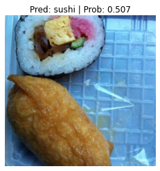
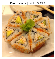
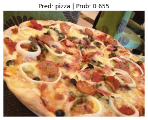
Those predictions look far better than the ones our TinyVGG model was previously making.

Making predictions on a custom image

It looks like our model does well qualitatively on data from the test set.

But how about on our own custom image?

That’s where the real fun of machine learning is!

Predicting on your own custom data, outisde of any training or test set.

To test our model on a custom image, let’s import the old faithful pizza-dad.jpeg image (an image of my dad eating pizza).

We’ll then pass it to the pred_and_plot_image() function we created above and see what happens.

# Download custom image
import requests

# Setup custom image path
custom_image_path = data_path / "04-pizza-dad.jpeg"

# Download the image if it doesn't already exist
if not custom_image_path.is_file():
    with open(custom_image_path, "wb") as f:
        # When downloading from GitHub, need to use the "raw" file link
        request = requests.get("images/04-pizza-dad.jpeg")
        print(f"Downloading {custom_image_path}...")
        f.write(request.content)
else:
    print(f"{custom_image_path} already exists, skipping download.")

# Predict on custom image
pred_and_plot_image(model=model,
                    image_path=custom_image_path,
                    class_names=class_names)

data/04-pizza-dad.jpeg already exists, skipping download.

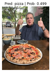
Two thumbs up!

Looks like our model got it right again!

But this time the prediction probability is higher than the one from TinyVGG (0.373) in PyTorch Custom Datasets section 11.3.

This indicates our efficientnet_b0 model is more confident in its prediction where as our TinyVGG model was par with just guessing.

Main takeaways

• Transfer learning often allows to you get good results with a relatively small amount of custom data.

• Knowing the power of transfer learning, it’s a good idea to ask at the start of every problem, “does an existing well-performing model exist for my problem?”

• When using a pretrained model, it’s important that your custom data be formatted/preprocessed in the same way that the original model was trained on, otherwise you may get degraded performance.

• The same goes for predicting on custom data, ensure your custom data is in the same format as the data your model was trained on.

• There are several different places to find pretrained models from the PyTorch domain libraries, HuggingFace Hub and libraries such as timm (PyTorch Image Models).

Extra-curriculum

• Look up what “model fine-tuning” is and spend 30-minutes researching different methods to perform it with PyTorch. How would we change our code to fine-tine? Tip: fine-tuning usually works best if you have lots of custom data, where as, feature extraction is typically better if you have less custom data.

• Check out the new/upcoming PyTorch multi-weights API (still in beta at time of writing, May 2022), it’s a new way to perform transfer learning in PyTorch. What changes to our code would need to made to use the new API?

• Try to create your own classifier on two classes of images, for example, you could collect 10 photos of your dog and your friends dog and train a model to classify the two dogs. This would be a good way to practice creating a dataset as well as building a model on that dataset.